A projectile with air resistance

A spherical projectile of mass $$m$$ launched with some initial velocity moves under the influence of two forces: gravity, $\boldsymbol{F}_g = -mg\boldsymbol{\hat{z}}$ , and air resistance (drag), $\boldsymbol{F}_D = -\frac{1}{2}c\rho A v^2 \boldsymbol{v}/|\boldsymbol{v}| = -\frac{1}{2}c\rho A v\boldsymbol{v}$ , acting in the opposite direction to the projectile's velocity and proportional to the square of that velocity (under most realistic conditions). Here, $$c$$ is the drag coefficient, $\rho$ the air density, and $$A$$ the projectile's cross-sectional area.

The relevant equations of motion are therefore:

\begin{align*} m\ddot{x} &= -k\sqrt{\dot{x}^2 + \dot{z}^2}\dot{x},\\ m\ddot{z} &= -k\sqrt{\dot{x}^2 + \dot{z}^2}\dot{z} - mg, \end{align*}

where $v = |\boldsymbol{v}| = \sqrt{\dot{x}^2 + \dot{z}^2}$ and $k=\frac{1}{2}c\rho A$ . These can be decomposed into the following four first-order ODEs with $u_1 \equiv x, u_2 \equiv \dot{x}, u_3 \equiv z, u_4 \equiv \dot{z}$ :

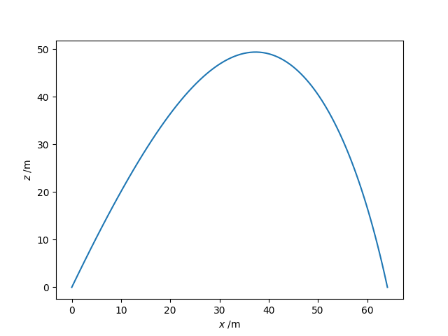
\begin{align*} \dot{u}_1 &= u_2,\\ \dot{u}_2 &= -\frac{k}{m}\sqrt{u_2^2 + u_4^2}u_2,\\ \dot{u}_3 &= u_4, \\ \dot{u}_4 &= -\frac{k}{m}\sqrt{u_2^2 + u_4^2}u_4 - g. \end{align*}

The following code integrates this system and identifies two events: hitting the target (the projectile returning to the ground at $$z=0$$ ) and reaching its maximum height (at which the z-component of its velocity is zero). We set the additional attribute hit_target.direction = -1 to ensure that hit_target only triggers the event when its return value (the projectile's elevation) goes from positive to negative; otherwise the event would be triggered at launch since $$z_0 = 0$$ . Other possibilities are direction = 1: trigger the event when the return value changes from negative to positive or direction = 0 (the default): the event is triggered when the return value is zero from either direction.

airresistance

import numpy as np
from scipy.integrate import solve_ivp
import matplotlib.pyplot as plt

# Drag coefficient, projectile radius (m), area (m2) and mass (kg).
c = 0.47
r = 0.05
A = np.pi * r**2
m = 0.2
# Air density (kg.m-3), acceleration due to gravity (m.s-2).
rho_air = 1.28
g = 9.81
# For convenience, define  this constant.
k = 0.5 * c * rho_air * A

# Initial speed and launch angle (from the horizontal).
v0 = 50
phi0 = np.radians(65)


def deriv(t, u):
    x, xdot, z, zdot = u
    speed = np.hypot(xdot, zdot)
    xdotdot = -k / m * speed * xdot
    zdotdot = -k / m * speed * zdot - g
    return xdot, xdotdot, zdot, zdotdot


# Initial conditions: x0, v0_x, z0, v0_z.
u0 = 0, v0 * np.cos(phi0), 0.0, v0 * np.sin(phi0)
# Integrate up to tf unless we hit the target sooner.
t0, tf = 0, 50


def hit_target(t, u):
    # We've hit the target if the z-coordinate is 0.
    return u[2]


# Stop the integration when we hit the target.
hit_target.terminal = True
# We must be moving downwards (don't stop before we begin moving upwards!)
hit_target.direction = -1


def max_height(t, u):
    # The maximum height is obtained when the z-velocity is zero.
    return u[3]


soln = solve_ivp(
    deriv, (t0, tf), u0, dense_output=True, events=(hit_target, max_height)
)
print(soln)
print(f"Time to target = {soln.t_events[0][0]:.2f} s")
print(f"Time to highest point = {soln.t_events[1][0]:.2f} s")

# A fine grid of time points from 0 until impact time.
t = np.linspace(0, soln.t_events[0][0], 100)

# Retrieve the solution for the time grid and plot the trajectory.
sol = soln.sol(t)
x, z = sol[0], sol[2]
print(f"Range to target, xmax = {x[-1]:.2f} m")
print(f"Maximum height, zmax = {max(z):.2f} m")
plt.plot(x, z)
plt.xlabel("$x$ /m")
plt.ylabel("$z$ /m")
plt.show()

The output is:

Time to target = 6.34 s
Time to highest point = 2.79 s
Range to target, xmax = 64.12 m
Maximum height, zmax = 49.42 m

and the plot created is shown in below.

The trajectory of a spherical projectile including air resistance.

E8.18A projectile with air resistance