The temperature dependence of resistivity

P6.X.5The temperature dependence of resistivity

The resistance of a wire of length $$l$$ and cross section area $$A$$ is given by $R = \rho l / A$ , where $\rho$ is the resisitivity (SI units: $\mathrm{\Omega\,m}$ ). Over reasonably narrow temperature ranges, $$R$$ increases with temperature linearly:

R(T) = R_0[1+\alpha(T-T_0)],

where $\alpha$ is a constant. Fit a straight line to the following data sets and determine $\rho$ for copper and iron at the reference temperature $T_0 = 300\;\mathrm{K}$ . The data are measured for a wire of circular cross sectional radius $0.1\;\mathrm{mm}$ and length $100\;\mathrm{m}$ .

$T\;/\mathrm{K}$	$R(\mathrm{Cu})\;/\mathrm{\Omega}$	$R(\mathrm{Fe})\;/\mathrm{\Omega}$
220.0	0.33	1.89
250.0	0.51	2.31
280.0	0.59	2.77
310.0	0.44	3.25
340.0	0.64	3.71
370.0	0.70	4.25
400.0	0.73	4.66

Show solution

Here is one solution, giving the following output:

rho(Cu) =  1.707e-08 Ω.m
rho(Fe) =  9.760e-08 Ω.m

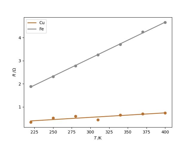
Two equivalent methods for fitting the straight line are given.

resistivity

import numpy as np
import matplotlib.pyplot as plt

# Reference temperature.
T0 = 300

# Wire radius (r, m), length (L, m) and cross sectional area (A, m2).
r, L = 1.0e-3, 100
A = np.pi * r**2

# The resistance data to fit.
R = {}
T, R["Cu"], R["Fe"] = np.array(
    [
        [220.0, 0.33, 1.89],
        [250.0, 0.51, 2.31],
        [280.0, 0.59, 2.77],
        [310.0, 0.44, 3.25],
        [340.0, 0.64, 3.71],
        [370.0, 0.70, 4.25],
        [400.0, 0.73, 4.66],
    ]
).T


def get_R(T, R0, alpha):
    """Return resistance, R, at temperature T."""
    return R0 * (1 + alpha * (T - T0))


def fit_line(x, y):
    """Linear fit as a simple degree-1 polynomial."""
    return np.polyfit(x, y, deg=1)


def fit_line(x, y):
    """Linear fit with linalg.lstsq."""
    n = len(x)
    A = np.vstack((x, np.ones(n))).T
    m, c = np.linalg.lstsq(A, y)[0]
    return m, c


# Perform the fit and plot the data points and best fit straight line.
fig, ax = plt.subplots()

colors = {"Cu": "#B87333", "Fe": "#888888"}
for metal in ("Cu", "Fe"):
    m, c = fit_line(T - T0, R[metal])
    R0, alpha = c, m / c
    rho = R0 * A / L
    print("rho({}) = {:10.3e} Ω.m".format(metal, rho))
    ax.plot(T, R[metal], "o", c=colors[metal])
    ax.plot(T, get_R(T, R0, alpha), "-", lw=2, c=colors[metal], label=metal)
ax.set_xlabel(r"$T\;/\mathrm{K}$")
ax.set_ylabel(r"$R\;/\mathrm{\Omega}$")
ax.legend(loc="best")

plt.show()