Modeling meanders · scipython.com

P6.6.4Modeling meanders

One way to simulate the meanders in a river is as the average of a large number of a random walks [1,2]. Using a coordinate system $$(x,y)$$ , start at point $$A = (0,0)$$ and aim to finish at $$B = (b,0)$$ . Starting from an initial heading of $\phi_0$ from the $$AB$$ direction, at each step change this angle by a random amount drawn from a normal distribition with mean $\mu=0$ and standard deviation $\sigma$ , and proceed by unit distance in this direction. Discard any walks which do not, after $$n$$ steps, finish within one unit of $$B$$ (this will be the majority!).

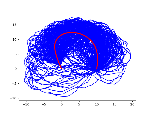
Write a program to find the average path meeting the above constraints for $$b=10$$ , using $\phi_0 = 110^\circ$ , $\sigma = 17^\circ$ , $$n=40$$ and $$10^6$$ random walk trials. Plot the accepted walks and their average, which should resemble a meander.

B. Hayes, American Scientist 94, 490 (2006).
H. von Schelling, General Electric Report No. 64GL92.

Show solution

The main part of the program below consists of two loops: each time around the outer loop over the number of trials we reset $\phi_0$ and the array of path positions, pos and conduct the random walk over $$n$$ steps (the inner loop). If, after a walk, we are within one unit of the end position, B, we add that walk to the average, plot it, and increment the counter for completed walks, ngood. Finally, we divide our accumulated paths by ngood to find the average path and plot that.

meanders

import numpy as np
import matplotlib.pyplot as plt

# Random walk from a = (0,0) to b = (b, 0)
b = 10
# Set off each time at an angle phi0 from the a-b direction
phi0 = np.radians(110)
# Take a total of 40 steps
n = 40
# At each step, change phi by a random amount selected from a normal
# distribution with standard deviation sigma
sigma = np.radians(17)

# Conduct a total of ntrials walks
ntrials = 1000000
av = np.zeros((n, 2))
ngood = 0
for j in range(ntrials):
    phi = phi0
    pos = np.zeros((n, 2))
    for i in range(1, n):
        dx, dy = np.cos(phi), np.sin(phi)
        pos[i] = pos[i - 1] + (dx, dy)
        phi += sigma * np.random.randn()
    if np.hypot(b - pos[-1, 0], pos[-1, 1]) < 1.0:
        plt.plot(pos[:, 0], pos[:, 1], color="b")
        av += pos
        ngood += 1
        print(j)
av /= ngood
plt.plot(av[:, 0], av[:, 1], lw=3, color="r")
plt.show()

A typical output is shown below.