P6.X.2Measuring the Coefficient of Restitution
The coefficient of restitution, \(C_\mathrm{R}\), of a ball dropped vertically onto a surface is the ratio of the ball's speed just before it hits the surface to its speed immediately after it bounces back from it. If the ball is dropped from a height \(h_0\) above the surface, it is easy to show that it will be travelling with speed \(v_0 = \sqrt{2g/h_0}\) when it hits; its speed as it bounces back up will then be \(v_1 = C_\mathrm{R}v_0\).
More generally, the upward speed of the ball after the \(n\)th bounce is:
An experiment to measure \(C_\mathrm{R}\), assuming it is independent of the ball's speed, may be conducted as follows. Drop the ball from a height \(h_0\) at time \(t=0\) and record the sound of the ball hitting the surface over a number of bounces. The time between the bounce events is then
(show this), where \(T_0 = 2v_0/g\). Then
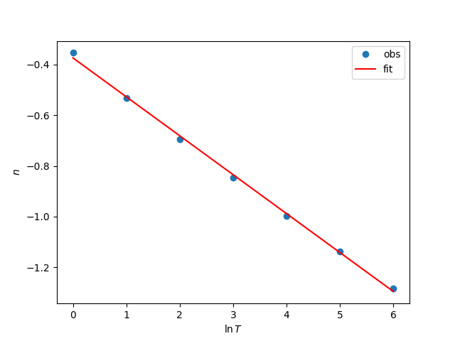
and so a plot of \(\ln T_n\) against \(n\) should be a straight line with gradient \(\ln C_\mathrm{R}\).
The data file bounce-data.txt is a text-version of the recording of an experiment carried out as described above, with a sampling frequency of \(4410\;\mathrm{s^{-1}}\) (i.e. data points are separated by \(1/4410\;\mathrm{s}\)). Analyse these data to find a value for \(C_\mathrm{R}\). If \(h_0 = 57.5\;\mathrm{cm}\), what is the value of \(g\) inferred from the intercept?
Show solution
The following program gives \(CR = 0.86\) and \(g = 9.7\;\mathrm{m\,s^{-1}}\).
import numpy as np
import matplotlib.pyplot as plt

data = np.loadtxt("bounce-data.txt")
fs = 4410  # sample rate (s-1)
n = len(data)
# Set up a time-grid
t = np.linspace(0, float(n) / fs, n)
# When the signal reaches <thresh>, count a bounce...
thresh = 0.05
# then skip the next <width> data points which are the sound of the bounce
width = 700

# make a list of bounce event times
bounce_time = []
i = 0
while i < n:
    if data[i] > thresh:
        bounce_time.append(t[i])
        i += width
    i += 1

# create a numpy array of the bounce time intervals
T = np.empty(len(bounce_time) - 1)
for i in range(len(T)):
    T[i] = bounce_time[i + 1] - bounce_time[i]

# we want to plot ln(T) vs n where n is the bounce number
lnT = np.log(T)
n = np.linspace(0, len(lnT) - 1, len(lnT))

# set up the linear equations lnT = m.n + c as the matrix
# equation lnT = Ap where p is (m, c)
A = np.vstack([n, np.ones(len(n))]).T
# find the "best" values of m, c by linear least squares fit
m, c = np.linalg.lstsq(A, lnT)[0]

# we're done: calculate CR and g from m and c
CR = np.exp(m)
T0 = np.exp(c)
h0 = 0.575
g = 8.0 * h0 / T0**2
print(CR, g)

# finally, plot the data and best fit line
plt.plot(n, lnT, "o", label="obs")
plt.plot(n, m * n + c, "r", label="fit")
plt.xlabel(r"$\ln T$")
plt.ylabel(r"$n$")
plt.legend()
plt.show()