P6.7.2Fourier expansion of a square wave
A square wave of period \(T\) may be defined through the following function:
with \(f(t) = f(t + nT)\) for \(n=\pm 1, \pm 2, \cdots\).
Plot the square wave with \(T=1\) (and hence cycle frequency, \(\nu=1\)) for \(0 \le t < 2\) taking a grid of 2048 time points over this interval. Calculate and plot its discrete Fourier Transform.
The Fourier expansion of this function is the infinite series
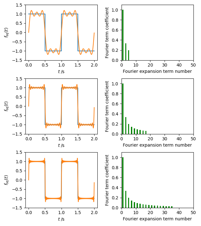
Compare the square wave function with this Fourier expansion truncated at 3, 9 and 18 terms. Also compare their (suitably normalized) Fourier transforms: the missing frequencies in each truncated series should appear as zeros in its Fourier transform, whereas the present terms will have intensities \(4/[\pi(2k-1)]\).
Show solution
The three cases are handled in the code below.
import numpy as np
import matplotlib.pyplot as plt

n = 2048
T = 1
freq = 1 / T
duration = 2
t = np.arange(0, duration, duration / n)
f = np.ones(n)
f[(t >= T / 2) & (t < T)] = -1
f[t >= T] = f[t < T]

# 3x2 subplots, with total figure size of 6.4" x 7.2".
fig, axes = plt.subplots(nrows=3, ncols=2, figsize=(6.4, 7.2))


def fourier_expansion(nterms):
    fourier_square = np.zeros(n)
    for k in range(1, nterms + 1):
        fac = 2 * k - 1
        fourier_square += np.sin(2 * np.pi * fac * freq * t) / fac
    return 4 / np.pi * fourier_square


for i, nterms in enumerate((3, 9, 18)):
    fourier_square = fourier_expansion(nterms)

    F = (duration / n) / (4 / np.pi) * np.abs(np.fft.rfft(fourier_square))
    Fdft = (duration / n) / (4 / np.pi) * np.abs(np.fft.rfft(f))
    Ffreq = np.fft.rfftfreq(n, duration / n)

    ax = axes[i, 0]
    ax.plot(t, f)
    ax.plot(t, fourier_square)
    ax.set_xlabel(r"$t\;/\mathrm{s}$")
    ax.set_ylabel(r"$f_\mathrm{sq}(t)$")
    ax.set_ylim(-1.5, 1.5)

    ax = axes[i, 1]
    ax.bar(Ffreq, F, color="g")
    ax.set_xlabel("Fourier expansion term number")
    ax.set_ylabel("Fourier term coefficient")
    ax.set_xlim(0, 50)
    ax.set_ylim(0, 1.1)

plt.tight_layout()
plt.show()
The plot produced by this code is shown below.