Numerical stability of an integral solved by recursion

The integral

I_n = \int_0^1 x^n e^x\,\mathrm{d}x \quad n=0,1,2,\cdots

suggests a recursion relation obtained by integration by parts:

I_n = \left[ x^n e^x \right]_0^1 - n\int_0^1x^{n-1}e^x\,\mathrm{d}x = e - nI_{n-1}

terminating with $$I_0 = e-1$$ . However, this algorithm, applied "forwards" for increasing $$n$$ is numerically unstable since small errors (such as floating point rounding errors) are magnified at each step: if the error in $$I_n$$ is $\epsilon_n$ such that the estimated value of $$I_n$$ is $I_n' + \epsilon_n$ then

\epsilon_n = I_n' - I_n = (e-nI_{n-1}') - (e - nI_{n-1}) = n(I_{n-1} - I_{n-1}') = -n\epsilon_{n-1},

and hence $|\epsilon_n| = n!\epsilon_{0}$ . Even if the error in $\epsilon_0$ is small, that in $\epsilon_n$ is larger by a factor $$n!$$ which can be huge.

The numerically stable solution, in this case, is to apply the recursion backwards for decreasing $$n$$ :

I_{n-1} = \frac{1}{n}(e - I_n) \quad \Rightarrow \epsilon_{n-1} = -\frac{\epsilon_n}{n}.

That is, errors in $$I_n$$ are reduced on each step of the recursion. One can even start the algorithm at $$I'_N = 0$$ and providing enough steps are taken between $$N$$ and the desired $$n$$ it will converge on the correct $$I_n$$ .

integralstability

import numpy as np
import matplotlib.pyplot as plt


def Iforward(n):
    if n == 0:
        return np.e - 1
    return np.e - n * Iforward(n - 1)


def Ibackward(n):
    if n >= 99:
        return 0
    return (np.e - Ibackward(n + 1)) / (n + 1)


N = 35
Iforward = [np.e - 1]
for n in range(1, N + 1):
    Iforward.append(np.e - n * Iforward[n - 1])

Ibackward = [0] * (N + 1)
for n in range(N - 1, -1, -1):
    Ibackward[n] = (np.e - Ibackward[n + 1]) / (n + 1)

n = range(N + 1)
plt.plot(n, Iforward, label="Forward algorithm")
plt.plot(n, Ibackward, label="Backward algorithm")
plt.ylim(-0.5, 2)
plt.xlabel("$n$")
plt.ylabel("$I(n)$")
plt.legend()
plt.show()

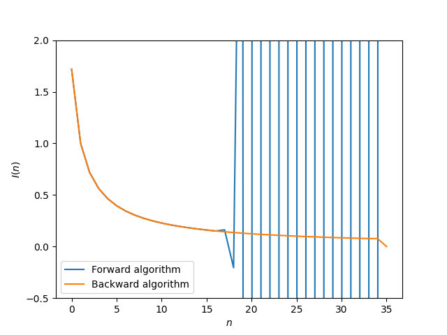
The figure below shows the forwards algorithm becoming extremely unstable for $$n>16$$ and fluctuating between very large positive and negative values; conversely, the backwards algorithm is well-behaved.

Numerical instability on forward algorithm.

E10.2Numerical stability of an integral solved by recursion