Learning Scientific Programming with Python (2nd edition)
E9.3: Data analysis: female literacy in India
The file india-data.csv, contains columns of demographic data on the 36 states and union territories (UTs) of India. When read in with:
In [x]: import pandas as pd
In [x]: import matplotlib.pyplot as plt
In [x]: df = pd.read_csv('india-data.csv', index_col=0)
the DataFrame produced contains an Index of State/UT name and columns:
In [x]: df.index
Out[x]:
Index(['Uttar Pradesh', 'Maharashtra', 'Bihar', 'West Bengal',
       ...
       'Dadra and Nagar Haveli', 'Daman and Diu', 'Lakshadweep'],
      dtype='object', name='State/UT')

In [x]: df.columns
Out[x]:
Index(['Male Population', 'Female Population', 'Area (km2)',
       'Male Literacy (%)', 'Female Literacy (%)', 'Fertility Rate'],
      dtype='object')
We can quickly inspect the DataFrame with df.head(n), which outputs the first n rows (or five rows if n is not specified):
In [x]: df.head()
Out[x]:
                Male Population  ...  Female Literacy (%)
State/UT                         ...
Uttar Pradesh         104480510  ...                59.26
Maharashtra            58243056  ...                75.48
Bihar                  54278157  ...                53.33
West Bengal            46809027  ...                71.16
Madhya Pradesh         37612306  ...                60.02

[5 rows x 5 columns]
pandas makes it straightforward to compute new columns for our DataFrame:
In [x]: df['Population'] = df['Male Population'] + df['Female Population']
In [x]: total_pop = df['Population'].sum()
In [x]: print(f'Total population: {total_pop:,d}')
Total population: 1,210,754,977

In [x]: df['Population Density (km-2)'] = df['Population'] / df['Area (km2)']
In [x]: df.loc['West Bengal', 'Population Density (km-2)']
Out[x]: 1028.440091490896       # population density of West Bengal

In [x]: total_pop / df['Area (km2)'].sum()
Out[x]: 368.3195047153525       # mean population density
Maximum and minimum values are obtained in the same way as in NumPy, for example:
In [x]: df['Male Literacy (%)'].min()
Out[x]: 73.39
Perhaps more usefully, idxmin and idxmax return the index label(s) of the minimum and maximum values, respectively:
In [x]: df['Area (km2)'].idxmax()   # largest state/UT by area
Out[x]: 'Rajasthan'
Naturally, the value returned can be passed to df.loc to obtain the entire row. For example, the row corresponding to the most densely populated State / UT:
In [x]: df.loc[df['Population Density (km-2)'].idxmax()]
Out[x]:
Male Population              8887326
Female Population            7800615
Area (km2)                   1484
Male Literacy (%)            91.03
Female Literacy (%)          80.93
Population                   16687940
Population Density (km-2)    1.124524e+04
Name: Delhi, dtype: float64
Correlation statistics between DataFrames or Series can be calculated with the corr function:
In [x]: df['Female Literacy (%)'].corr(df['Fertility Rate'])
Out[x]: -0.7361949271996956
In this case (two columns of data being compared), a single correlation coefficient is produced. More generally, the correlation matrix is returned as a new DataFrame. pandas can be used to quickly produce a variety of simple, labeled plots and charts from a DataFrame with a family of df.plot methods. By default, these use the Matplotlib backend, so the syntax is the same as presented in Chapter 7. For example,
In [x]: df.plot.scatter('Female Literacy (%)', 'Fertility Rate')
In [x]: plt.show()
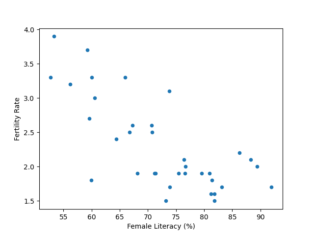
Scatter plot of fertility rate against female literacy for the 36 States and UTs of India.