Learning Scientific Programming with Python (2nd edition)
E8.25: Weighted and non-weighted least-squares fitting
To illustrate the use of curve_fit in weighted and unweighted least squares fitting, the following program fits the Lorentzian line shape function centered at $x_0$ with halfwidth at half-maximum (HWHM), $\gamma$, amplitude, $A$:
$$
f(x) = \frac{A \gamma^2}{\gamma^2 + (x-x_0)^2},
$$
to some artificial noisy data. The fit parameters are $A$, $\gamma$ and $x_0$. The noise is such that a region of the data close to the line centre is much noisier than the rest.
import numpy as np
from scipy.optimize import curve_fit
import matplotlib.pyplot as plt

x0, A, gamma = 12, 3, 5

n = 200
x = np.linspace(1, 20, n)
yexact = A * gamma**2 / (gamma**2 + (x - x0) ** 2)

# Add some noise with a sigma of 0.5 apart from a particularly noisy region
# near x0 where sigma is 3
sigma = np.ones(n) * 0.5
sigma[np.abs(x - x0 + 1) < 1] = 3
noise = np.random.randn(n) * sigma
y = yexact + noise


def f(x, x0, A, gamma):
    """The Lorentzian entered at x0 with amplitude A and HWHM gamma."""
    return A * gamma**2 / (gamma**2 + (x - x0) ** 2)


def rms(y, yfit):
    return np.sqrt(np.sum((y - yfit) ** 2))


# Unweighted fit
p0 = 10, 4, 2
popt, pcov = curve_fit(f, x, y, p0)
yfit = f(x, *popt)
print("Unweighted fit parameters:", popt)
print("Covariance matrix:")
print(pcov)
print("rms error in fit:", rms(yexact, yfit))
print()

# Weighted fit
popt2, pcov2 = curve_fit(f, x, y, p0, sigma=sigma, absolute_sigma=True)
yfit2 = f(x, *popt2)
print("Weighted fit parameters:", popt2)
print("Covariance matrix:")
print(pcov2)
print("rms error in fit:", rms(yexact, yfit2))

plt.plot(x, yexact, label="Exact")
plt.errorbar(
    x,
    y,
    yerr=np.abs(noise),
    elinewidth=0.5,
    c="gray",
    marker="+",
    lw=0,
    label="Noisy data",
)
plt.plot(x, yfit, label="Unweighted fit")
plt.plot(x, yfit2, label="Weighted fit")
plt.ylim(-1, 4)
plt.legend(loc="lower center")
plt.show()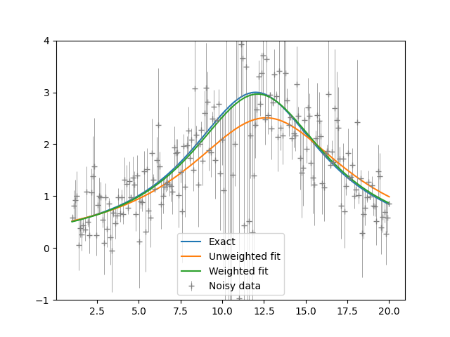
Weighted and unweighted least-squares fitting to a Lorentzian function.
As the figure above shows, the unweighted fit is seen to be thrown off by the noisy region. Data in this region are given a lower weight in the weighted fit and so the parameters are closer to their true values and the fit better. The output is:
Unweighted fit parameters: [12.61968131  2.50893152  5.95025464]
Covariance matrix:
[[ 0.17447292 -0.0042928   0.04156738]
 [-0.0042928   0.03051659 -0.09208499]
 [ 0.04156738 -0.09208499  0.54308245]]
rms error in fit: 3.737100164521528

Weighted fit parameters: [12.12134294  2.96625048  5.05555878]
Covariance matrix:
[[ 0.02135293 -0.00360315  0.0078179 ]
 [-0.00360315  0.01100727 -0.02128371]
 [ 0.0078179  -0.02128371  0.06642836]]
rms error in fit: 0.49516367688465607