Learning Scientific Programming with Python (2nd edition)
E8.9: The Voigt profile
The Voigt line profile occurs in the modelling and analysis of radiative transfer in the atmosphere. It is the convolution of a Gaussian profile, $G(x; \sigma)$ and a Lorentzian profile, $L(x; \gamma)$: $$ \begin{align*} V(x; \sigma, \gamma) = \int_{-\infty}^\infty G(x';\sigma)L(x-x';\gamma)\,\mathrm{d}x' \quad\mathrm{where}\\ G(x;\sigma) = \frac{1}{\sigma\sqrt{2\pi}}\exp\left(-\frac{x^2}{2\sigma^2}\right) \quad \mathrm{and}\quad L(x;\gamma) = \frac{\gamma/\pi}{x^2 + \gamma^2}. \end{align*} $$ Here $\gamma$ is the half-width at half-maximum (HWHM) of the Lorentzian profile and $\sigma$ is the standard deviation of the Gaussian profile, related to its HWHM, $\alpha$, by $\alpha = \sigma\sqrt{2\ln 2}$. In terms of frequency, $\nu$, $x = \nu - \nu_0$ where $\nu_0$ is the line centre.
There is no closed form for the Voigt profile, but it is related to the real part of the Faddeeva function, $w(z)$ by $$ V(x;\sigma,\gamma) = \frac{\renewcommand\Re{\operatorname{Re}}\Re{[w(z)]}}{\sigma\sqrt{2\pi}}, \;\mathrm{where}\;z = \frac{x + i\gamma}{\sigma\sqrt{2}}. $$
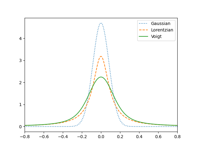
The program below plots the Voigt profile for $\gamma = 0.1, \alpha = 0.1$ and compares it with the corresponding Gaussian and Lorentzian profiles. The equations above are implemented in the three functions, G, L and V defined in the code below.
import numpy as np
from scipy.special import wofz
import matplotlib.pyplot as plt


def G(x, alpha):
    """Return Gaussian line shape at x with HWHM alpha"""
    return (
        np.sqrt(np.log(2) / np.pi)
        / alpha
        * np.exp(-((x / alpha) ** 2) * np.log(2))
    )


def L(x, gamma):
    """Return Lorentzian line shape at x with HWHM gamma"""
    return gamma / np.pi / (x**2 + gamma**2)


def V(x, alpha, gamma):
    """
    Return the Voigt line shape at x with Lorentzian component HWHM gamma
    and Gaussian component HWHM alpha.

    """
    sigma = alpha / np.sqrt(2 * np.log(2))

    return (
        np.real(wofz((x + 1j * gamma) / sigma / np.sqrt(2)))
        / sigma
        / np.sqrt(2 * np.pi)
    )


alpha, gamma = 0.1, 0.1
x = np.linspace(-0.8, 0.8, 1000)
plt.plot(x, G(x, alpha), ls=":", label="Gaussian")
plt.plot(x, L(x, gamma), ls="--", label="Lorentzian")
plt.plot(x, V(x, alpha, gamma), label="Voigt")
plt.xlim(-0.8, 0.8)
plt.legend()
plt.show()
Comparison of the Gaussian, Lorentzian and Voigt profiles.