Learning Scientific Programming with Python (2nd edition)
E8.16: Stokes drag
An object falling slowly in a viscous fluid under the influence of gravity is subject to a drag force (Stokes drag) which varies linearly with its velocity. Its equation of motion may be written as the second order differential equation: $$ m\frac{\mathrm{d}^2z}{\mathrm{d}t^2} = -c \frac{\mathrm{d}z}{\mathrm{d}t} + mg', $$ where $z$ is the object's position as a function of time, $t$, $c$ is a drag constant which depends on the shape of the object and the fluid viscosity, and $$ g' = g\left(1-\frac{\rho_\mathrm{fluid}}{\rho_\mathrm{obj}}\right) $$ is the effective gravitational acceleration, which accounts for the buoyant force due to the fluid (density $\rho_\mathrm{fluid}$) displaced by the object (density $\rho_\mathrm{obj}$). For a small sphere of radius $r$ in a fluid of viscosity $\eta$, Stokes' law predicts $c = 6\pi\eta r$.
Consider a sphere of platinum ($\rho = 21.45\;\mathrm{g\,cm^{-3}}$) with radius 1 mm, initially at rest, falling in mercury ($\rho = 13.53\;\mathrm{g\,cm^{-3}}$, $\eta = 1.53 \times 10^{-3}\;\mathrm{Pa\,s}$). The above second-order differential equation can be solved analytically, but to integrate it numerically using odeint, it must be treated as two first-order ordinary differential equations:
$$
\begin{align*}
\frac{\mathrm{d}z}{\mathrm{d}t} &= \dot{z}\\
\frac{\mathrm{d}^2z}{\mathrm{d}t^2} = \frac{\mathrm{d}\dot{z}}{\mathrm{d}t} &= g' - \frac{c}{m}\dot{z}
\end{align*}
$$
In the code below, the function deriv calculates these derivatives and is passed to odeint with the intial conditions ($z=0$, $\dot{z}=0$) and a grid of time points.
import numpy as np
from scipy.integrate import solve_ivp
import matplotlib.pyplot as plt

# Platinum sphere falling from rest in mercury.

# Acceleration due to gravity (m.s-2).
g = 9.81
# Densities (kg.m-3).
rho_Pt, rho_Hg = 21450, 13530
# Viscosity  of mercury (Pa.s).
eta = 1.53e-3

# Radius and mass of the sphere.
r = 1.0e-3  # radius (m)
m = 4 * np.pi / 3 * r**3 * rho_Pt
# Drag constant from Stokes' law.
c = 6 * np.pi * eta * r
# Effective gravitational acceleration.
gp = g * (1 - rho_Hg / rho_Pt)


def deriv(t, z):
    """Return the dz/dt and d2z/dt2."""
    dz0 = z[1]
    dz1 = gp - c / m * z[1]
    return dz0, dz1


t0, tf = 0, 20
t_eval = np.linspace(t0, tf, 50)
# Initial conditions: z = 0, dz/dt = 0 at t = 0.
z0 = (0, 0)

# Integrate the pair of differential equations.
sol = solve_ivp(deriv, (t0, tf), z0, t_eval=t_eval)
t = sol.t
z, zdot = sol.y
plt.plot(t, zdot)

print("Estimate of terminal velocity = {:.3f} m.s-1".format(zdot[-1]))

# Exact solution: terminal velocity vt (m.s-1) and characteristic time tau (s).
v0, vt, tau = 0, m * gp / c, m / c
print("Exact terminal velocity = {:.3f} m.s-1".format(vt))
z = (
    vt * t
    + v0 * tau * (1 - np.exp(-t / tau))
    + vt * tau * (np.exp(-t / tau) - 1)
)
zdot_exact = vt + (v0 - vt) * np.exp(-t / tau)
plt.plot(t, zdot_exact)
plt.xlabel(r"$t$ /s")
plt.ylabel(r"$\dot{z}\;/\mathrm{m\, s^{-1}}$")
plt.show()
The plot produced by this program is shown below: the numerical and analytical results are indistinguishable at this scale but are reported to three decimal places in the output:
Estimate of terminal velocity = 11.266 m.s-1
Exact terminal velocity = 11.285 m.s-1
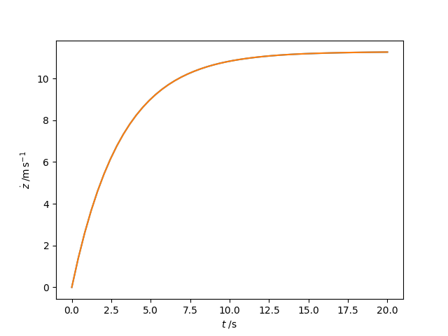
Velocity of a platinum sphere falling in mercury.