Solving a system of stiff ODEs

A classic example of a stiff system of ODEs is the kinetic analysis of Robertson's autocatalytic chemical reaction: H. H. Robertson, The solution of a set of reaction rate equations, in J. Walsh (Ed.), Numerical Analysis: An Introduction, pp. 178–182, Academic Press, London (1966).

The reaction involves three species, $x=[\mathrm{X}]$ , $y=[\mathrm{Y}]$ and $z=[\mathrm{Z}]$ with initial conditions $x=1$ , $y=z=0$ :

$\begin{align*} \dot{x} \equiv \frac{\mathrm{d}x}{\mathrm{d}t} &= -0.04x + 10^4yz,\\ \dot{y} \equiv \frac{\mathrm{d}y}{\mathrm{d}t} &= 0.04x - 10^4yz - 3 \times 10^7 y^2,\\ \dot{z} \equiv \frac{\mathrm{d}z}{\mathrm{d}t} &= 3 \times 10^7 y^2. \end{align*}$ (Note the very different timescales of the reactions, particularly for $[\mathrm{Y}]$ .)

With the default Runge–Kutta algorithm on the time interval $[0, 500]$ :

def deriv(t, y):
    x, y, z = y
    xdot = -0.04 * x + 1.e4 * y * z
    ydot = 0.04 * x - 1.e4 * y * z - 3.e7 * y**2
    zdot = 3.e7 * y**2
    return xdot, ydot, zdot

t0, tf = 0, 500
y0 = 1, 0, 0
soln = solve_ivp(deriv, (t0, tf), y0)
print(soln)

We get there eventually:

  message: 'The solver successfully reached the end of the integration interval.'
     nfev: 6123410
     njev: 0
      nlu: 0
      sol: None
   status: 0
  success: True
        t: array([0.00000000e+00, 6.36669332e-04, 1.06518798e-03, ...,
       4.99999288e+02, 4.99999819e+02, 5.00000000e+02])
 t_events: None
        y: array([[1.00000000e+00, 9.99974534e-01, 9.99957394e-01, ...,
        4.19780946e-01, 4.19780771e-01, 4.19780487e-01],
       [0.00000000e+00, 2.20107324e-05, 3.00616449e-05, ...,
        2.41400796e-06, 2.47838908e-06, 2.72514279e-06],
       [0.00000000e+00, 3.45561028e-06, 1.25439771e-05, ...,
        5.80216640e-01, 5.80216750e-01, 5.80216788e-01]])

but at the cost of more than 6 million function evaluations (soln.nfev). The 'Radau' method fares much better:

import numpy as np
from scipy.integrate import solve_ivp
import matplotlib.pyplot as plt

def deriv(t, y):
    """ODEs for Robertson's chemical reaction system."""
    x, y, z = y
    xdot = -0.04 * x + 1.e4 * y * z
    ydot = 0.04 * x - 1.e4 * y * z - 3.e7 * y**2
    zdot = 3.e7 * y**2
    return xdot, ydot, zdot

# Initial and final times.
t0, tf = 0, 500
# Initial conditions: [X] = 1; [Y] = [Z] = 0.
y0 = 1, 0, 0
# Solve, using a method resilient to stiff ODEs.
soln = solve_ivp(deriv, (t0, tf), y0, method='Radau')
print(soln.nfev, 'evaluations required.')

# Plot the concentrations as a function of time. Scale [Y] by 10**YFAC
# so its variation is visible on the same axis used for [X] and [Z].
YFAC = 4
plt.plot(soln.t, soln.y[0], label='[X]')
plt.plot(soln.t, 10**YFAC*soln.y[1], label=r'$10^{}\times$[Y]'.format(YFAC))
plt.plot(soln.t, soln.y[2], label='[Z]')
plt.xlabel('time /s')
plt.ylabel('concentration /arb. units')
plt.legend()
plt.show()

The output indicates only 248 evaluations required. The concentrations of $[\mathrm{X}]$ , $[\mathrm{Y}]$ and $[\mathrm{Z}]$ are plotted against time below.

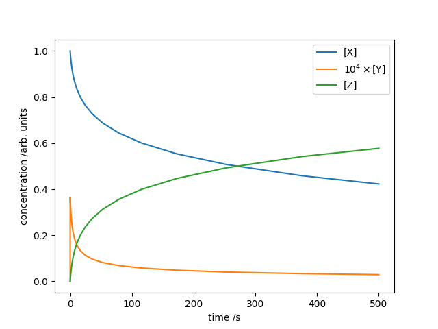
The Robertson chemical equation system, numerically integrated with the Radau IIA method