Learning Scientific Programming with Python (2nd edition)
E7.12: Modelling an antenna array
An antenna array can be used to direct radio waves in a particular direction by adjusting their number, geometrical arrangement, and relative amplitudes and phases (see e.g. S. J. Orfanidis, Electromagnetic Waves and Antennas, Rutgers University, 2016.)
Consider an array of $n$ isotropic antennas at positions, $\boldsymbol{d}_i$, evenly spaced by $d$ along the $x$-axis from the origin:
$$ \begin{align*} \boldsymbol{d}_0 = 0, \boldsymbol{d}_1 = d\boldsymbol{\hat{x}}, \ldots,\boldsymbol{d}_{n-1} = (n-1)d\boldsymbol{\hat{x}}. \end{align*} $$
If a single antenna produces a radiation vector, $\boldsymbol{F}(\boldsymbol{k})$, where $\boldsymbol{k} = k\boldsymbol{\hat{r}} = (2\pi/\lambda)\boldsymbol{\hat{r}}$, the total radiation vector due to all $n$ antennas is
$$ \begin{align*} \boldsymbol{F}_\mathrm{tot}(\boldsymbol{k}) = \sum_{j=0}^{n-1}w_j\mathrm{e}^{ji\boldsymbol{k}\cdot\boldsymbol{d}_j}\boldsymbol{F}(\boldsymbol{k}) = A(\boldsymbol{k})F(\boldsymbol{k}), \end{align*} $$
where $w_j$ is the feed coefficient of the $j$th antenna, representing its amplitude and phase, and $A(\boldsymbol{k})$ is known as the array factor. We can choose $w_0 = 1$ to specify the feed coefficients relative to the antenna at the origin. If we further choose to look only at the azimuthal ($\phi$) contribution to the radiation in the $xy$ plane, setting the polar angle $\theta=\pi/2$, we have: $$ A(\phi) = \sum_{j=0}^{n-1}w_j\mathrm{e}^{jikd\cos\phi}. $$
The relative radiation power pattern ("gain") is the square of this quantity. For two identical antennas, $$ g(\phi) = |A(\phi)|^2 = |w_0 + w_1\mathrm{e}^{ikd\cos\phi}|^2. $$ In the code below, the related quantity, the directive gain, $10\log_{10}(g/g_\mathrm{max})$, is plotted below as a function of $\phi$ for the two-antenna case on a polar plot for $d=\lambda$ and $w_0 =1, w_1 = -i$.
import numpy as np
import matplotlib.pyplot as plt


def gain(d, w):
    """Return the power as a function of azimuthal angle, phi."""
    phi = np.linspace(0, 2 * np.pi, 1000)
    psi = 2 * np.pi * d / lam * np.cos(phi)
    A = w[0] + w[1] * np.exp(1j * psi)
    g = np.abs(A) ** 2
    return phi, g


def get_directive_gain(g, minDdBi=-20):
    """Return the "directive gain" of the antenna array producing gain g."""
    DdBi = 10 * np.log10(g / np.max(g))
    return np.clip(DdBi, minDdBi, None)


# Wavelength, antenna spacing, feed coefficients.
lam = 1
d = lam
w = np.array([1, -1j])
# Calculate gain and directive gain; plot on a polar chart.
phi, g = gain(d, w)
DdBi = get_directive_gain(g)

plt.polar(phi, DdBi, c="k", lw=2)
ax = plt.gca()
ax.set_rticks([-20, -15, -10, -5])
ax.set_rlabel_position(45)
plt.show()
Notes:
- To better show the interesting region of the plot, where the power is highest, we "clip" the values less than
minDdBito that value. - To customize the plot we need the Axes object in the current plot context; this is returned by
plt.gca()("get current axes"). set_rtickssets the position of the radial tick marks.set_rlabel_positiondefines the angular position of the radial ticks.
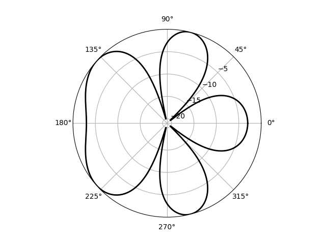
The directive gain of a two-antenna array with $d = \lambda, w_0 = 1; w_1 = -i$.
NumPy's broadcasting methods provide a natural way to extend this code to an arbitrary number of antennas; in the following example the figure method add_subplot is called with the argument projection='polar' and returns a corresponding Axes object, ax.
import numpy as np
import matplotlib.pyplot as plt


def gain(d, w):
    """Return the power as a function of azimuthal angle, phi."""
    phi = np.linspace(0, 2 * np.pi, 1000)
    psi = 2 * np.pi * d / lam * np.cos(phi)
    j = np.arange(len(w))
    A = np.sum(w[j] * np.exp(j * 1j * psi[:, None]), axis=1)
    g = np.abs(A) ** 2
    return phi, g


def get_directive_gain(g, minDdBi=-20):
    """Return the "directive gain" of the antenna array producing gain g."""
    DdBi = 10 * np.log10(g / np.max(g))
    return np.clip(DdBi, minDdBi, None)


# Wavelength, antenna spacing, feed coefficients.
lam = 1
d = lam / 2
w = np.array([1, -1, 1])
# Calculate gain and directive gain; plot on a polar chart.
phi, g = gain(d, w)
DdBi = get_directive_gain(g)

fig = plt.figure()
ax = fig.add_subplot(projection="polar")
ax.plot(phi, DdBi, c="k", lw=2)
ax.set_rticks([-20, -15, -10, -5])
ax.set_rlabel_position(45)
plt.show()
The sum to calculate $A$ is over the terms in the array factor expression: adding an axis to thepsi array calculates this sum for each of the angular positions, $\phi$.
Note that with the projection already defined, we need ax.plot here, not ax.polar to plot the data.
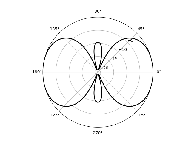
The directive gain of a many-antenna array with $d = \lambda/2, w_0 = 1;w_1 = -1;w_2 = 1$.