Learning Scientific Programming with Python (2nd edition)
E7.28: Animating a decaying sine curve 1
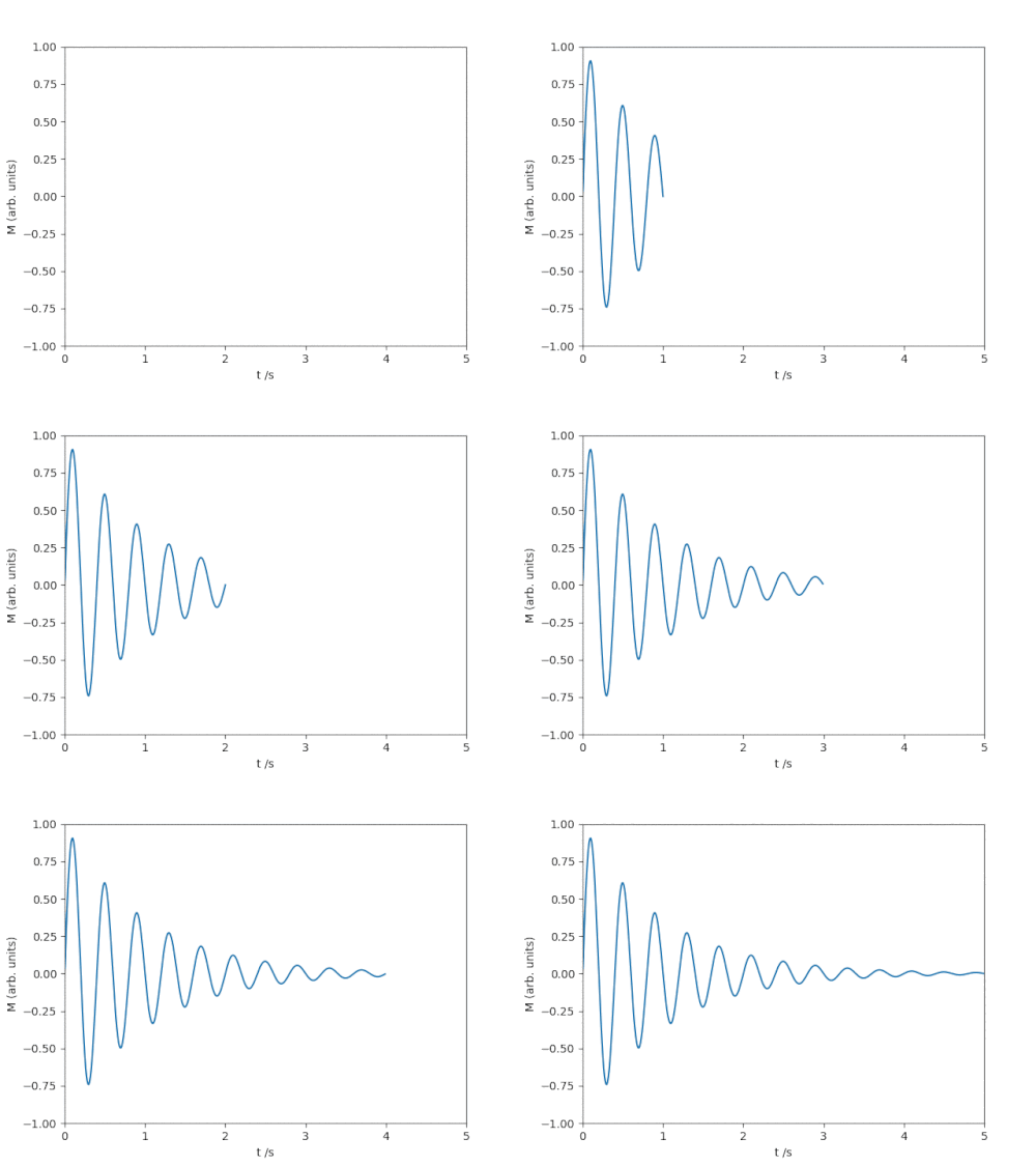
The following code animates a decaying sine curve that could, for example, represent the decaying chime of a struck tuning fork at a fixed frequency: $$ M(t) = \sin(2\pi f t)\mathrm{e}^{-\alpha t} $$
import numpy as np
import matplotlib.pyplot as plt
import matplotlib.animation as animation

# Time step for the animation (s), max time to animate for (s).
dt, tmax = 0.01, 5
# Signal frequency (s-1), decay constant (s-1).
f, alpha = 2.5, 1
# These lists will hold the data to plot.
t, M = [], []

# Draw an empty plot, but preset the plot x- and y-limits.
fig, ax = plt.subplots()
(line,) = ax.plot([], [])
ax.set_xlim(0, tmax)
ax.set_ylim(-1, 1)
ax.set_xlabel("t /s")
ax.set_ylabel("M (arb. units)")


def animate(i):
    """Draw the frame i of the animation."""

    global t, M
    # Append this time point and its data and set the plotted line data.
    _t = i * dt
    t.append(_t)
    M.append(np.sin(2 * np.pi * f * _t) * np.exp(-alpha * _t))
    line.set_data(t, M)


# Interval between frames in ms, total number of frames to use.
interval, nframes = 1000 * dt, int(tmax / dt)
# Animate once (set repeat=False so the animation doesn't loop).
ani = animation.FuncAnimation(
    fig, animate, frames=nframes, repeat=False, interval=interval
)
plt.show()- Recall that the
ax.plotmethod returns a tuple ofLine2Dobjects, even if there is only one plotted line. We need to retain a reference to it so we can set its data in the animation function,animate. - By declaring the
tandMlists to beglobalobjects we can modify them from inside theanimatefunction. - By setting the time interval between frames to be the same (in milliseconds) as the time step, the animation is made to appear "in real time."

Matplotlib animation of a ringdown process.