Learning Scientific Programming with Python (2nd edition)
E10.1: Numerical stability of the forward-Euler method
Consider the differential equation, $$ \frac{\mathrm{d}y}{\mathrm{d}x} = -\alpha y $$ for $\alpha > 0$ subject to the boundary condition $y(0)=1$. This simple problem can be solved analytically: $$ y = e^{-\alpha x}, $$ but suppose we want to solve it numerically. The simplest approach is the forward (or explicit) Euler method: choose a step-size, $h$, defining a grid of $x$ values, $x_i = x_{i-1} + h$, and approximate the corresponding $y$ values through: $$ y_i = y_{i-1} + h\left| \frac{\mathrm{d}y}{\mathrm{d}x} \right|_{x_{i-1}} = y_{i-1} - h\alpha y_{i-1} = y_{i-1}(1-\alpha h). $$ The question arises: what value should be chosen for $h$? A small $h$ minimises the error introduced by the approximation above which basically joins $y$ values by straight-line segments (that is, the Taylor series about $y_{i-1}$ has been truncated at the linear term in $h$). But if $h$ is too small there will be cancellation errors due to the finite precision used in representing the numbers involved. In the extreme case that $h$ is chosen to be smaller than the machine epsilon, typically about $2 \times 10^{-16}$, then we have $x_i = x_{i-1}$ and there is no grid of points at all.
The following code implements the forward Euler algorithm to solve the above differential equation.
import numpy as np
import matplotlib.pyplot as plt

alpha, y0, xmax = 2, 1, 10


def euler_solve(h, n):
    """Solve dy/dx = -alpha.y by forward Euler method for step size h."""
    y = np.zeros(n)
    y[0] = y0
    for i in range(1, n):
        y[i] = (1 - alpha * h) * y[i - 1]
    return y


def plot_solution(h):
    x = np.arange(0, xmax, h)
    y = euler_solve(h, len(x))
    plt.plot(x, y, label="$h={}$".format(h), lw=1)


for h in (0.01, 0.2, 1):
    plot_solution(h)

plt.legend()
plt.show()
The largest value of $h$ (here, $h = \alpha/2 = 1$) clearly makes the algorithm unstable.
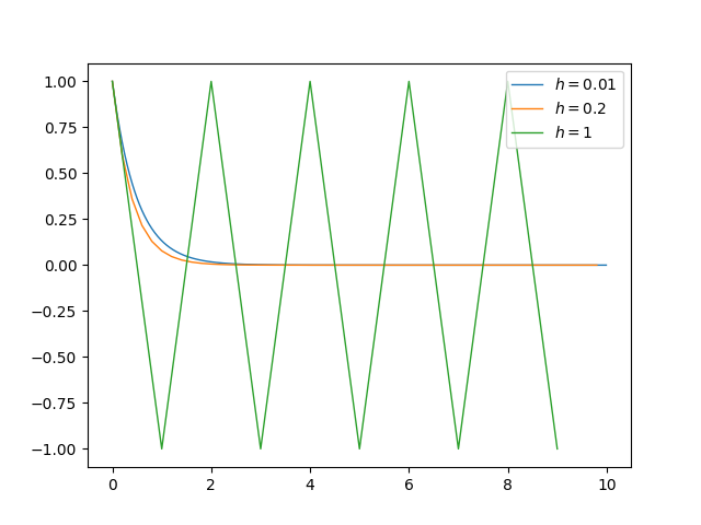
Numerical instability of the forward Euler method.