Learning Scientific Programming with Python (2nd edition)
E7.24: The two-dimensional diffusion equation
The two-dimensional diffusion equation is $$ \frac{\partial U}{\partial t} = D\left(\frac{\partial^2U}{\partial x^2} + \frac{\partial^2U}{\partial y^2}\right) $$ where $D$ is the diffusion coefficient. A simple numerical solution on the domain of the unit square $0\le x < 1, 0 \le y < 1$ approximates $U(x,y;t)$ by the discrete function $u_{i,j}^{(n)}$ where $x=i\Delta x$, $y=j\Delta y$ and $t=n\Delta t$. Applying finite difference approximations yields $$ \frac{u_{i,j}^{(n+1)} - u_{i,j}^{(n)}}{\Delta t} = D\left[ \frac{u_{i+1,j}^{(n)} - 2u_{i,j}^{(n)} + u_{i-1,j}^{(n)}}{(\Delta x)^2} + \frac{u_{i,j+1}^{(n)} - 2u_{i,j}^{(n)} + u_{i,j-1}^{(n)}}{(\Delta y)^2} \right], $$ and hence the state of the system at time step $n+1$, $u_{i,j}^{(n+1)}$ may be calculated from its state at time step $n$, $u_{i,j}^{(n)}$ through the equation $$ u_{i,j}^{(n+1)} = u_{i,j}^{(n)} + D\Delta t\left[ \frac{u_{i+1,j}^{(n)} - 2u_{i,j}^{(n)} + u_{i-1,j}^{(n)}}{(\Delta x)^2} + \frac{u_{i,j+1}^{(n)} - 2u_{i,j}^{(n)} + u_{i,j-1}^{(n)}}{(\Delta y)^2} \right]. $$
Consider the diffusion equation applied to a metal plate initially at temperature $T_\mathrm{cold}$ apart from a disc of a specified size which is at temperature $T_\mathrm{hot}$. We suppose that the edges of the plate are held fixed at $T_\mathrm{cool}$. The following code applies the above formula to follow the evolution of the temperature of the plate. It can be shown that the maximum time step, $\Delta t$ that we can allow without the process becoming unstable is $$ \Delta t = \frac{1}{2D}\frac{(\Delta x\Delta y)^2}{(\Delta x)^2 + (\Delta y)^2}. $$
In the code below, each call to do_timestep updates the numpy array u from the results of the previous timestep, u0. The simplest approach to applying the partial difference equation is to use a Python loop:
for i in range(1, nx-1):
    for j in range(1, ny-1):
        uxx = (u0[i+1,j] - 2*u0[i,j] + u0[i-1,j]) / dx2
        uyy = (u0[i,j+1] - 2*u0[i,j] + u0[i,j-1]) / dy2
        u[i,j] = u0[i,j] + dt * D * (uxx + uyy)
However, this runs extremely slowly and using vectorization will farm out these explicit loops to the much faster pre-compiled C-code underlying NumPy's array implementation.
import numpy as np
import matplotlib.pyplot as plt

# plate size, mm
w = h = 10.0
# intervals in x-, y- directions, mm
dx = dy = 0.1
# Thermal diffusivity of steel, mm2.s-1
D = 4.0

Tcool, Thot = 300, 700

nx, ny = int(w / dx), int(h / dy)

dx2, dy2 = dx * dx, dy * dy
dt = dx2 * dy2 / (2 * D * (dx2 + dy2))

u0 = Tcool * np.ones((nx, ny))
u = u0.copy()

# Initial conditions - circle of radius r centred at (cx,cy) (mm)
r, cx, cy = 2, 5, 5
r2 = r**2
for i in range(nx):
    for j in range(ny):
        p2 = (i * dx - cx) ** 2 + (j * dy - cy) ** 2
        if p2 < r2:
            u0[i, j] = Thot


def do_timestep(u0, u):
    # Propagate with forward-difference in time, central-difference in space.
    u[1:-1, 1:-1] = u0[1:-1, 1:-1] + D * dt * (
        (u0[2:, 1:-1] - 2 * u0[1:-1, 1:-1] + u0[:-2, 1:-1]) / dx2
        + (u0[1:-1, 2:] - 2 * u0[1:-1, 1:-1] + u0[1:-1, :-2]) / dy2
    )

    u0 = u.copy()
    return u0, u


# Number of timesteps.
nsteps = 101
# Output 4 figures at these timesteps.
mfig = [0, 10, 50, 100]
fignum = 0
fig, axes = plt.subplots(nrows=2, ncols=2)
for m in range(nsteps):
    u0, u = do_timestep(u0, u)
    if m in mfig:
        print(m, fignum)
        ax = axes[fignum // 2, fignum % 2]
        im = ax.imshow(
            u.copy(),
            cmap="hot",
            vmin=Tcool,
            vmax=Thot,
            interpolation="bilinear",
        )
        ax.set_axis_off()
        ax.set_title("{:.1f} ms".format(m * dt * 1000))
        fignum += 1
fig.subplots_adjust(right=0.85)
cbar_ax = fig.add_axes([0.9, 0.15, 0.03, 0.7])
cbar_ax.set_xlabel("$T$ / K", labelpad=20)
fig.colorbar(im, cax=cbar_ax)
plt.show()
To set a common colorbar for the four plots we define its own Axes, cbar_ax and make room for it with fig.subplots_adjust. The plots all use the same colour range, defined by vmin and vmax, so it doesn't matter which one we pass in the first argument to fig.colorbar.
The state of the system is plotted as an image at four different stages of its evolution.
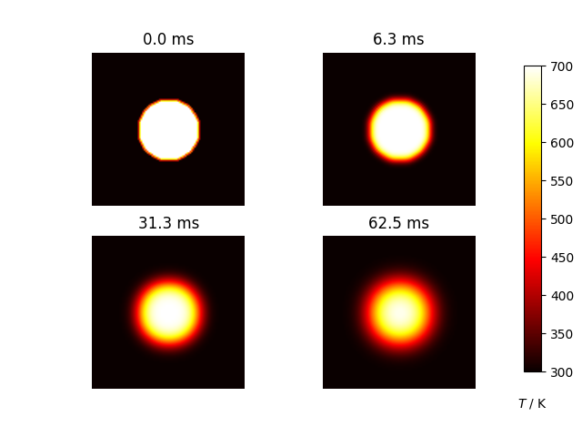
The two-dimensional diffusion equation.
Many thanks to Tim Teatro whose blog post inspired this example.