The ticker timer, much used in school physics experiments, is a device that marks dots on a strip of paper tape at evenly-spaced intervals of time as the tape moves through it at some (possibly variable) speed. The following data relate to the positions (in cm) of marks on a tape pulled through a ticker timer by a falling weight. The marks are made every 1/10 sec.
x = [1.3, 6.0, 20.2, 43.9, 77.0, 119.6, 171.7, 233.2, 304.2, 384.7,
474.7, 574.1, 683.0, 801.3, 929.2, 1066.4, 1213.2, 1369.4, 1535.1,
1710.3, 1894.9]
Fit these data to the function $x = x_0 + v_0t + \frac{1}{2}gt^2$ and determine an approximate value for the acceleration due to gravity, $g$.
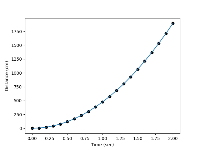
The following code fits the coefficients to the required quadratic equation. Note that this is a linear least squares fit even though the function is non-linear in time because it is linear with respect to the coefficients.
import numpy as np
import pylab
Polynomial = np.polynomial.Polynomial
x = np.array([1.3, 6.0, 20.2, 43.9, 77.0, 119.6, 171.7, 233.2, 304.2,
384.7, 474.7, 574.1, 683.0, 801.3, 929.2, 1066.4, 1213.2,
1369.4, 1535.1, 1710.3, 1894.9])
dt, n = 0.1, len(x)
tmax = dt * (n-1)
t = np.linspace(0, tmax, n)
A = np.vstack((np.ones(n), t, t**2)).T
coefs, resid, _, _ = np.linalg.lstsq(A, x)
# Initial position (cm) and speed (cm.s-1), acceleration due to gravity (m.s-2)
x0, v0, g = coefs[0], coefs[1], coefs[2] * 2 / 100
print('x0 = {:.2f} cm, v0 = {:.2f} cm.s-1, g = {:.2f} m.s-2'.format(x0, v0, g))
xfit = Polynomial(coefs)(t)
pylab.plot(t, x, 'ko')
pylab.plot(t, xfit, 'r')
pylab.xlabel('Time (sec)')
pylab.ylabel('Distance (cm)')
pylab.show()
The output and fitted function is shown below.
x0 = 1.28 cm, v0 = -0.04 cm.s-1, g = 9.47 m.s-2