Finding a best-fit straight line

Learning Scientific Programming with Python (2nd edition)

E6.12: Finding a best-fit straight line

A straight-line best fit is just a special case of a polynomial least-squares fit (with deg=1). Consider the following data giving the absorbance over a path length of 55 mm of UV light at 280 nm, $A$, by a protein as a function of the concentration, $[\mathrm{P}]$:

$[P] / \mathrm{\mu g.mL^{-1}}$	$A$
0	2.287
20	3.528
40	4.336
80	6.909
120	8.274
180	12.855
260	16.085
400	24.797
800	49.058
1500	89.400

We expect the absorbance to be linearly related to the protein concentration: $A = m[\mathrm{P}] + A_0$ where $A_0$ is the absorbance in the absence of protein (for example, due to the solvent and experimental components).

import numpy as np
import matplotlib.pyplot as plt

Polynomial = np.polynomial.Polynomial

# The data: conc = [P] and absorbance, A
conc = np.array([0, 20, 40, 80, 120, 180, 260, 400, 800, 1500])
A = np.array(
    [2.287, 3.528, 4.336, 6.909, 8.274, 12.855, 16.085, 24.797, 49.058, 89.400]
)

cmin, cmax = min(conc), max(conc)
pfit, stats = Polynomial.fit(
    conc, A, 1, full=True, window=(cmin, cmax), domain=(cmin, cmax)
)

print("Raw fit results:", pfit, stats, sep="\n")

A0, m = pfit
resid, rank, sing_val, rcond = stats
rms = np.sqrt(resid[0] / len(A))

print(f"Fit: A = {m:.3f}[P] + {A0:.3f}(rms residual = {rms:.4f})")

plt.plot(conc, A, "o")
plt.plot(conc, pfit(conc))
plt.xlabel(r"[P] /$\mathrm{\mu g\cdot mL^{-1}}$")
plt.ylabel("Absorbance")
plt.show()

The output shows a good straight-line fit to the data:

Raw fit results:
poly([ 1.92896129  0.0583057 ])
[array([ 2.47932733]), 2, array([ 1.26633786,  0.62959385]), 2.2204460492503131e-15]
Fit: A = 0.058[P] + 1.929 (rms residual = 0.4979)

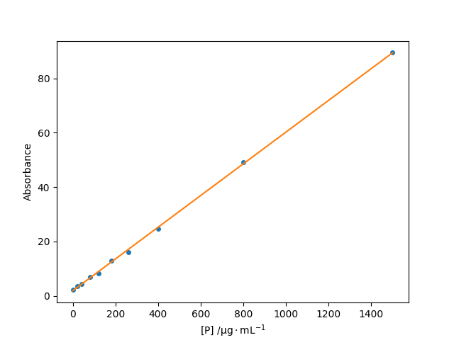
A best fit line to light absorbance as a function of protein concentration.