Blurring an image with a two-dimensional FFT

Learning Scientific Programming with Python (2nd edition)

E6.23: Blurring an image with a two-dimensional FFT

Note that there is an entire SciPy subpackage, scipy.ndimage, devoted to image processing. This example serves simply to illustrate the syntax and format of NumPy's two-dimensional FFT implementation.

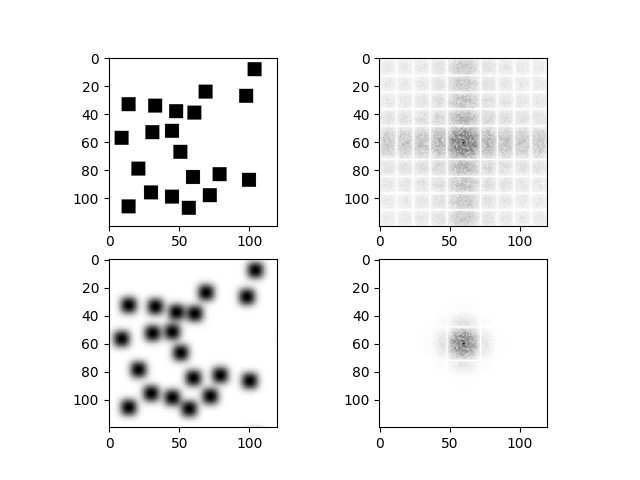
The two-dimensional DFT is widely-used in image processing. For example, multiplying the DFT of an image by a two-dimensional Gaussian function is a common way to blur an image by decreasing the magnitude of its high-frequency components.

The following code produces an image of randomly-arranged squares and then blurs it with a Gaussian filter.

import numpy as np
import matplotlib.pyplot as plt

# image size, square side length, number of squares
ncols, nrows = 120, 120
sq_size, nsq = 10, 20

# The image array (0=background, 1=square) and boolean array of allowed places
# to add a square so that it doesn't touch another or the image sides
image = np.zeros((nrows, ncols))
sq_locs = np.zeros((nrows, ncols), dtype=bool)
sq_locs[1 : -sq_size - 1 :, 1 : -sq_size - 1] = True


def place_square():
    """Place a square at random on the image and update sq_locs."""
    # valid_locs is an array of the indices of True entries in sq_locs
    valid_locs = np.transpose(np.nonzero(sq_locs))
    # pick one such entry at random, and add the square so its top left
    # corner is there; then update sq_locs
    i, j = valid_locs[np.random.randint(len(valid_locs))]
    image[i : i + sq_size, j : j + sq_size] = 1
    imin, jmin = max(0, i - sq_size - 1), max(0, j - sq_size - 1)
    sq_locs[imin : i + sq_size + 1, jmin : j + sq_size + 1] = False


# Add the required number of squares to the image
for i in range(nsq):
    place_square()
plt.imshow(image)
plt.show()

# Take the 2-dimensional DFT and centre the frequencies
ftimage = np.fft.fft2(image)
ftimage = np.fft.fftshift(ftimage)
plt.imshow(np.abs(ftimage))
plt.show()


# Build and apply a Gaussian filter.
sigmax, sigmay = 10, 10
cy, cx = nrows / 2, ncols / 2
x = np.linspace(0, nrows, nrows)
y = np.linspace(0, ncols, ncols)
X, Y = np.meshgrid(x, y)
gmask = np.exp(-(((X - cx) / sigmax) ** 2 + ((Y - cy) / sigmay) ** 2))

ftimagep = ftimage * gmask
plt.imshow(np.abs(ftimagep))
plt.show()

# Finally, take the inverse transform and show the blurred image
imagep = np.fft.ifft2(ftimagep)
plt.imshow(np.abs(imagep))
plt.show()

Blurring an image with FFT — Blurring an image using its Fast Fourier Transform. The original and blurred images appear on the lefthand side here, with their Fourier Transforms on the right.