What happens to carbon dioxide dissolved in water?
Posted on 11 June 2018
Carbon dioxide ($\mathrm{CO_2}$) dissolves in water, and some of the dissolved $\mathrm{CO_2}$ forms carbonic acid, $\mathrm{H_2CO_3(aq)}$: $$ \mathrm{CO_2(g)} + \mathrm{H_2O(l)} \rightleftharpoons \mathrm{H_2CO_3(aq)}. $$ This acid can then dissociate to form bicarbonate, $\mathrm{HCO_3^-}$: $$ K_1: \mathrm{H_2CO_3(aq)} \rightleftharpoons \mathrm{HCO_3^-(aq)} + \mathrm{H^+(aq)}, $$ which may further dissociate to carbonate, $\mathrm{CO_3^{2-}}$: $$ K_2: \mathrm{HCO_3^-(aq)} \rightleftharpoons \mathrm{CO_3^{2-}(aq)} + \mathrm{H^+(aq)}. $$
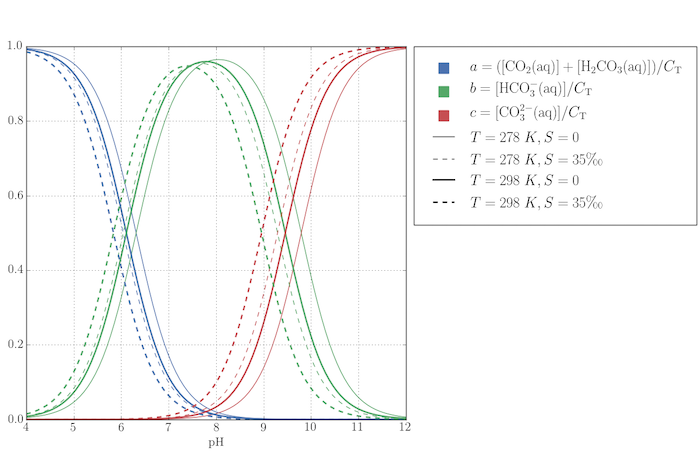
The degree of dissociation (the equilibrium constants for the above processes) determines the distribution of dissolved carbon amongst these species. It is useful to consider three quantities representing the species: $$ \begin{align*} a &= ([\mathrm{CO_2(aq)}] + [\mathrm{H_2CO_3(aq)}])/ C_\mathrm{T},\\ b &= [\mathrm{HCO_3^-(aq)}]/ C_\mathrm{T},\\ c &= [\mathrm{CO_3^{2-}(aq)}]/ C_\mathrm{T}, \end{align*} $$ where $C_\mathrm{T}=a+b+c$ is the total amount of dissolved carbon. With this convention, it is found that: $$ \begin{align*} a &= \frac{[\mathrm{H^+}]^2}{[\mathrm{H^+}]^2 + [\mathrm{H^+}]K_1 + K_1K_2},\\ b &= \frac{[\mathrm{H^+}]K_1}{[\mathrm{H^+}]^2 + [\mathrm{H^+}]K_1 + K_1K_2},\\ c &= \frac{K_1K_2}{[\mathrm{H^+}]^2 + [\mathrm{H^+}]K_1 + K_1K_2}.\\ \end{align*} $$
Empirical formulae are given here (pdf) for the equilbrium constants $K_1$ and $K_2$ which vary with temperature, $T$, and water salinity, $S$.
The script below plots the quantities $a$, $b$, and $c$ as a function of pH (and hence $[\mathrm{H^+}]$) for two different temperatures and freshwater ($S=0$) and average seawater ($S$ = 35 ‰). The pH range is wildly greater than would be expected for most bodies of water on Earth, however. Across the range of typical seawater pH, $7.5-8.4$, almost all the dissolved carbon that isn't $\mathrm{CO_2(aq)}$ is $\mathrm{HCO_3^-(aq)}$.
Some work is necessary to customize the legend in this figure: a custom HandlerPatch class creates the sqaure legend keys (which are rectangles by default), and some dummy lines are plotted to add the four types of labelled line styles.
import numpy as np
import matplotlib.pyplot as plt
from matplotlib.patches import Patch, Rectangle
from matplotlib.legend_handler import HandlerPatch

class HandlerSquare(HandlerPatch):
    """A Handler for creating square legend keys.

    See https://stackoverflow.com/a/27841028/293594 and
    https://matplotlib.org/users/legend_guide.html#implementing-a-custom-legend-handler

    """

    def create_artists(self, legend, orig_handle,
                       xdescent, ydescent, width, height, fontsize, trans):
        center = xdescent + 0.5 * (width - height), ydescent
        patch = Rectangle(xy=center, width=height,
                               height=height, angle=0.0)
        self.update_prop(patch, orig_handle, legend)
        patch.set_transform(trans)
        return [patch]

# Use LaTeX throughout the figure for consistency
plt.rc('font', **{'family': 'serif', 'serif': ['Computer Modern'], 'size': 16})
plt.rc('text', usetex=True)
# We need this package to use the per-mille symbol, ‰
plt.rc('text.latex', preamble=r'\usepackage{textcomp}')
# Figure dpi
dpi = 72

# Plot the amounts of dissolved carbon as CO2(aq) + H2CO3(aq), HCO3-(aq) and
# CO3-2(aq) (as fractions of the total carbon amount) as a function of pH for
# the two different temperatures and two different salinities.

def fK1p(T, S):
    """Equilibrium constant for H2CO3(aq) <-> H+(aq) + HCO3-(aq)

    T is the temperature (K) and S the salinity in parts per thousand.

    """

    pK1p = 3670.7/T - 62.008 + 9.7944*np.log(T) - 0.0118*S + 0.000116*S**2
    return 10**-pK1p

def fK2p(T, S):
    """Equilibrium constant for HCO3-(aq) <-> H+(aq) + CO3-2.

    T is the temperature (K) and S the salinity in parts per thousand.

    """

    pK2p = 1394.7/T + 4.777 - 0.0184*S + 0.000118*S**2
    return 10**-pK2p

def calc_C(H, T, S):
    """Calculate the fractional amounts of carbon as a function of [H+].

    T is the temperature (K) and S the salinity in parts per thousand.
    Returns a = ([CO2(aq)] + [H2CO3(aq)])/CT, b = [HCO3-(aq)]/CT, and
    c = [CO3-2(aq)]/CT, where CT is the total amount of dissolved carbon.


    """
    K1, K2 = fK1p(T, S), fK2p(T, S)
    K1K2 = K1*K2
    den = H * (H + K1) + K1K2
    a = H**2 / den
    b = H * K1 / den
    c = K1K2 / den
    return a, b, c

pH = np.linspace(4,12,100)
H = 10**-pH
T1, T2 = 278, 298
S1, S2 = 0, 35

colours = '#4c72b0', '#55a868', '#c64e52'
def plot_curves(ax, T, S, lw, ls):
    a, b, c = calc_C(H, T, S)
    ax.plot(pH, a, colours[0], lw=lw, ls=ls)
    ax.plot(pH, b, colours[1], lw=lw, ls=ls)
    ax.plot(pH, c, colours[2], lw=lw, ls=ls)

fig = plt.figure(figsize=(900/dpi, 600/dpi), dpi=dpi)
ax = fig.add_subplot(111)
plot_curves(ax, T1, S1, 1, '-')
plot_curves(ax, T2, S1, 2, '-')
plot_curves(ax, T1, S2, 1, '--')
plot_curves(ax, T2, S2, 2, '--')

ax.set_xlabel('pH')

# Make a custom legend box for the plot.
legend_handles = [
    Patch(color=colours[0], label='$a = ([\mathrm{CO_2(aq)}] +'
            ' [\mathrm{H_2CO_3(aq)}])/ C_\mathrm{T}$'),
    Patch(color=colours[1], label='$b = [\mathrm{HCO_3^-(aq)}] /'
            ' C_\mathrm{T}$'),
    Patch(color=colours[2], label='$c = [\mathrm{CO_3^{2-}(aq)}] /'
            ' C_\mathrm{T}$'),
    plt.Line2D((0,1),(0,0), color='k', lw=1, ls='-',
                    label='$T={}\;K, S={}$'.format(T1, S1)),
    plt.Line2D((0,1),(0,0), color='k', lw=1, ls='--',
                    label='$T={}\;K, S={}$\\textperthousand'.format(T1, S2)),
    plt.Line2D((0,1),(0,0), color='k', lw=2, ls='-',
                    label='$T={}\;K, S={}$'.format(T2, S1)),
    plt.Line2D((0,1),(0,0), color='k', lw=2, ls='--',
                    label='$T={}\;K, S={}$\\textperthousand'.format(T2, S2))
]
# Put the legend out of the Axes on the righthand side of the plot
ax = plt.gca()
box = ax.get_position()
# Move the plot Axes left to make room for the legend
ax.set_position([box.x0*0.3, box.y0, box.width*0.7, box.height])
# When bbox_to_anchor and loc are used together, loc identifies which point
# on the legend box is anchored at bbox_to_anchor in fractional Axes coords;
# borderaxespad is the padding between the anchor point and the legend box,
# borderpad is the padding inside the legend box. Both are in multiples of the
# font size (i.e. about an em).
ax.legend(handles=legend_handles, bbox_to_anchor=(1.02,1), loc='upper left',
          borderaxespad=0, borderpad=1,
          #handler_map={legend_handles[0]: HandlerSquare(), legend_handles[1]: HandlerSquare(), legend_handles[2]: HandlerSquare()}
          handler_map=dict(zip(legend_handles[:3], [HandlerSquare()]*3)) )
ax.grid('on')

plt.savefig('CaCO3_eqm.png')
plt.show()