Visualizing the Earth's dipolar magnetic field
Posted on 28 August 2019
The magnetic field due to a magnetic dipole moment, $\boldsymbol{m}$ at a point $\boldsymbol{r}$ relative to it may be written $$ \boldsymbol{B}(\boldsymbol{r}) = \frac{\mu_0}{4\pi r^3}[3\boldsymbol{\hat{r}(\boldsymbol{\hat{r}} \cdot \boldsymbol{m}) - \boldsymbol{m}}], $$ where $\mu_0$ is the vacuum permeability. In geomagnetism, it is usual to write the radial and angular components of $\boldsymbol{B}$ as: $$ \begin{align*} B_r & = -2B_0\left(\frac{R_\mathrm{E}}{r}\right)^3\cos\theta, \\ B_\theta & = -B_0\left(\frac{R_\mathrm{E}}{r}\right)^3\sin\theta, \\ B_\phi &= 0, \end{align*} $$ where $\theta$ is polar (colatitude) angle (relative to the magnetic North pole), $\phi$ is the azimuthal angle (longitude), and $R_\mathrm{E}$ is the Earth's radius, about 6370 km. See below for a derivation of these formulae.
With this definition, $B_0$ denotes the magnitude of the mean value of the field at the magnetic equator on the Earth's surface, about $31.2\; \mathrm{\mu T}$.
With these definitions, we can plot the dipole component of the Earth's magnetic field as a Matplotlib streamplot. We first construct a meshgrid of $(x,y)$ coordinates and convert them into polar coordinates with the relations:
$$
\begin{align*}
r &= \sqrt{x^2 + y^2},\\
\theta &= \mathrm{atan2}(y/x),
\end{align*}
$$
where the two-argument arctangent function, $\mathrm{atan2}$, is implemented in NumPy as arctan2. We can then use the formulae above to calculate $B_r$ and $B_\theta$ and convert back to Cartesian coordinates to plot the streamplot. The $\theta$ coordinate is offset by $\alpha = 9.6^\circ$ to account for the current tilt of the Earth's magnetic dipole with respect to its rotational axis.
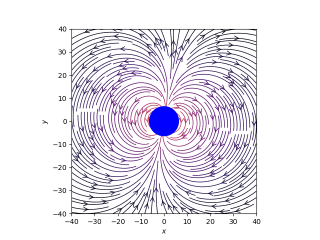
import sys
import numpy as np
import matplotlib.pyplot as plt
from matplotlib.patches import Circle

# Mean magnitude of the Earth's magnetic field at the equator in T
B0 = 3.12e-5
# Radius of Earth, Mm (10^6 m: mega-metres!)
RE = 6.370
# Deviation of magnetic pole from axis
alpha = np.radians(9.6)

def B(r, theta):
    """Return the magnetic field vector at (r, theta)."""
    fac = B0 * (RE / r)**3
    return -2 * fac * np.cos(theta + alpha), -fac * np.sin(theta + alpha)

# Grid of x, y points on a Cartesian grid
nx, ny = 64, 64
XMAX, YMAX = 40, 40
x = np.linspace(-XMAX, XMAX, nx)
y = np.linspace(-YMAX, YMAX, ny)
X, Y = np.meshgrid(x, y)
r, theta = np.hypot(X, Y), np.arctan2(Y, X)

# Magnetic field vector, B = (Ex, Ey), as separate components
Br, Btheta = B(r, theta)
# Transform to Cartesian coordinates: NB make North point up, not to the right.
c, s = np.cos(np.pi/2 + theta), np.sin(np.pi/2 + theta)
Bx = -Btheta * s + Br * c
By = Btheta * c + Br * s

fig, ax = plt.subplots()

# Plot the streamlines with an appropriate colormap and arrow style
color = 2 * np.log(np.hypot(Bx, By))
ax.streamplot(x, y, Bx, By, color=color, linewidth=1, cmap=plt.cm.inferno,
              density=2, arrowstyle='->', arrowsize=1.5)

# Add a filled circle for the Earth; make sure it's on top of the streamlines.
ax.add_patch(Circle((0,0), RE, color='b', zorder=100))

ax.set_xlabel('$x$')
ax.set_ylabel('$y$')
ax.set_xlim(-XMAX, XMAX)
ax.set_ylim(-YMAX, YMAX)
ax.set_aspect('equal')
plt.show()
Derivation
For now, consider the dipole to lie along the $y$-axis: $\boldsymbol{m} = m\boldsymbol{\hat{\jmath}}$ and define $\boldsymbol{B_0}$ to be the field perpendicular to $\boldsymbol{m}$ at a distance $R_\mathrm{E}$ from it (i.e. on the Earth's magnetic equator): $$ \boldsymbol{B_0} = -\frac{\mu_0m}{4\pi R_\mathrm{E}^3} \boldsymbol{\hat{\jmath}} = B_0\boldsymbol{\hat{\jmath}}. $$ Then, $$ \boldsymbol{B}(\boldsymbol{r}) = -B_0 \left(\frac{R_\mathrm{E}}{r}\right)^3 [3\cos\theta \boldsymbol{\hat{r}} - \boldsymbol{\hat{\jmath}}]. $$ The radial component of the magnetic field is therefore $$ B_r = \boldsymbol{B}\cdot\boldsymbol{\hat{r}} = -B_0\left(\frac{R_\mathrm{E}}{r}\right)^3[3\cos\theta - \cos\theta] = -2B_0\left(\frac{R_\mathrm{E}}{r}\right)^3\cos\theta, $$ Its angular component is perpendicular to this: $$ B_\theta = \boldsymbol{B}\cdot\boldsymbol{\hat{\theta}} = - B_0 \left(\frac{R_\mathrm{E}}{r}\right)^3 [-\boldsymbol{\hat{\jmath}} \cdot \boldsymbol{\hat{\theta}}] = -B_0\left(\frac{R_\mathrm{E}}{r}\right)^3\sin\theta. $$ Finally, $B_\phi = 0$: the field is symmetric about the axis of the dipole.
Further Reading
- Wikipedia article on the dipole model of the Earth's magnetic field
- M. Walt, Introduction to Geomagnetically Trapped Radiation (1994), Cambridge University Press.