The Wilberforce Pendulum

The Wilberforce Pendulum is a mass suspended on a helical spring which is free to move up and down as well as to rotate as the spring coils and uncoils with its extension. You can see one in action below.

An analysis of the motion of a Wilberforce pendulum was carried out by Berg and Marshall ["Wilberforce pendulum oscillations and normal modes", Am. J. Phys. 59 (1991)] who give the following Lagrangian equations of motion for the extension, $z$, and torsion, $\theta$ of the spring:

\begin{align*} m\frac{\mathrm{d}^2z}{\mathrm{d}t^2} + kz + \frac{1}{2}\epsilon\theta & = 0,\\ I\frac{\mathrm{d}^2\theta}{\mathrm{d}t^2} + \delta\theta + \frac{1}{2}\epsilon z & = 0, \end{align*}

where $k$ and $\delta$ are the longitudinal and torsional spring constants respectively and $m$ and $I$ are the mass and moment of inertia of the suspended bob. $\epsilon$ is the coupling constant between the linear and twisting motions.

These equations may be put into canonical form as \begin{align*} \frac{\mathrm{d}\dot{z}}{\mathrm{d}t} = -\omega^2z - \frac{\epsilon}{2m}\theta & \quad \frac{\mathrm{d}z}{\mathrm{d}t} = \dot{z},\\ \frac{\mathrm{d}\dot{\theta}}{\mathrm{d}t} = -\omega^2\theta - \frac{\epsilon}{2I}z & \quad \frac{\mathrm{d}\theta}{\mathrm{d}t} = \dot{\theta}, \end{align*} where $\omega = \omega_z = \omega_\theta$ for resonance between the two modes with frequencies $\omega_z = \sqrt{k/m}$ and $\omega_\theta = \sqrt{\delta/I}$.

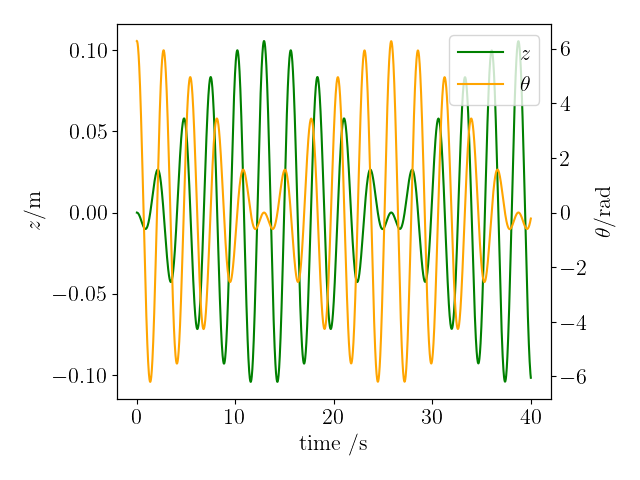
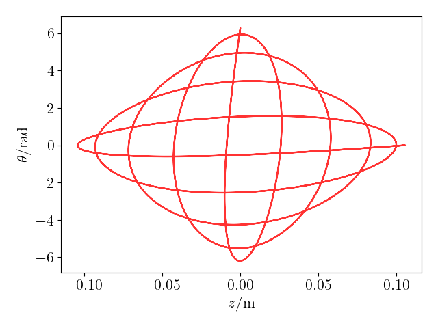
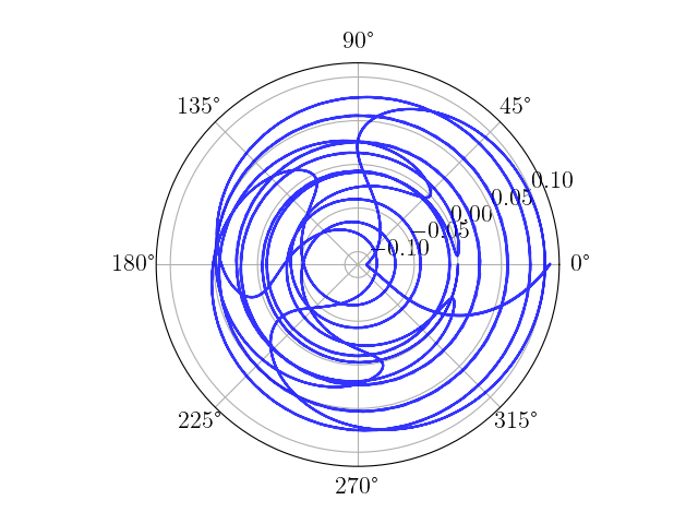
To simulate this system using SciPy, we use scipy.integrate.solve_ivp in the code below, which generates plots of $z$ and $\theta$ against time as well as cartesian and polar plots of $z$ against $\theta$.

import numpy as np
from scipy.integrate import solve_ivp
from matplotlib import rc
import matplotlib.pyplot as plt
import matplotlib

# Plot parameters related to the Wilberforce pendulum
# Mathematical details are available on my blog article,
# at https://scipython.com/blog/the-wilberforce-pendulum/
# Christian Hill, January 2016.
# Updated (January 2020) to use solve_ivp instead of odeint.

# Use LaTeX throughout the figure for consistency.
rc('font', **{'family': 'serif', 'serif': ['Computer Modern'], 'size': 16})
rc('text', usetex=True)

# Parameters for the system
omega = 2.314       # rad.s-1
epsilon = 9.27e-3   # N
m = 0.4905          # kg
I = 1.39e-4         # kg.m2

def deriv(t, y, omega, epsilon, m, I):
    """Return the first derivatives of y = z, zdot, theta, thetadot."""
    z, zdot, theta, thetadot = y
    dzdt = zdot
    dzdotdt = -omega**2 * z - epsilon / 2 / m * theta
    dthetadt = thetadot
    dthetadotdt = -omega**2 * theta - epsilon / 2 / I * z
    return dzdt, dzdotdt, dthetadt, dthetadotdt

# Initial conditions: theta=2pi, z=zdot=thetadot=0
y0 = [0, 0, 2*np.pi, 0]

# Do the numerical integration of the equations of motion up to tmax secs.
tmax = 40
soln = solve_ivp(deriv, (0, tmax), y0, args=(omega, epsilon, m, I), dense_output=True)
# The time grid in s
t = np.linspace(0, tmax, 2000)
# Unpack z and theta as a function of time
z, theta = soln.sol(t)[0], soln.sol(t)[2]

# Plot z vs. t and theta vs. t on axes which share a time (x) axis
fig, ax_z = plt.subplots()
l_z, = ax_z.plot(t, z, 'g', label=r'$z$')
ax_z.set_xlabel('time /s')
ax_z.set_ylabel(r'$z /\mathrm{m}$')
ax_theta = ax_z.twinx()
l_theta, = ax_theta.plot(t, theta, 'orange', label=r'$\theta$')
ax_theta.set_ylabel(r'$\theta /\mathrm{rad}$')

# Add a single legend for the lines of both twinned axes
lines = (l_z, l_theta)
labels = [line.get_label() for line in lines]
plt.legend(lines, labels)
plt.savefig('wilberforce_z-t_plot.png')
plt.show()

# Plot theta vs. z on a cartesian plot
fig, ax1 = plt.subplots()
ax1.plot(z, theta, 'r', alpha=0.8)
ax1.set_xlabel(r'$z /\mathrm{m}$')
ax1.set_ylabel(r'$\theta /\mathrm{rad}$')
plt.tight_layout()
plt.savefig('wilberforce_theta-z_plot.png')
plt.show()

# Plot z vs. theta on a polar plot
fig, ax2 = plt.subplots(subplot_kw={'projection': 'polar'})
ax2.plot(theta, z, 'b', alpha=0.8)
plt.savefig('wilberforce_theta-z_polar_plot.png')
plt.show()

Comments

Comments are pre-moderated. Please be patient and your comment will appear soon.

Jose Luis Castro 7 years, 6 months ago

Es un gran trabajo
experimental
teorico
y computacional !!!

Link | Reply

christian 7 years, 6 months ago

Muchas gracias – I'm glad you found it interesting.

Calixto 3 years ago

Hi! Can you provide a code solving the same problem but now using the fourth-order Runge-Kutta Method? I am having so much trouble and I hope you will be able to help me out. Thank you!

christian 3 years ago

The default integration method used by solve_ivp is the explicit Runge-Kutta method of order 5(4).