A simple model of a polymer in solution treats its monomer units as totally uncorrelated in position (each monomer unit adopts a random orientation with respect to all the others): this is the random flight model.

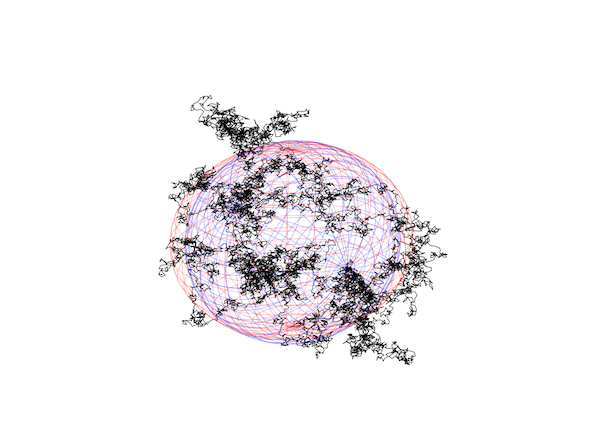
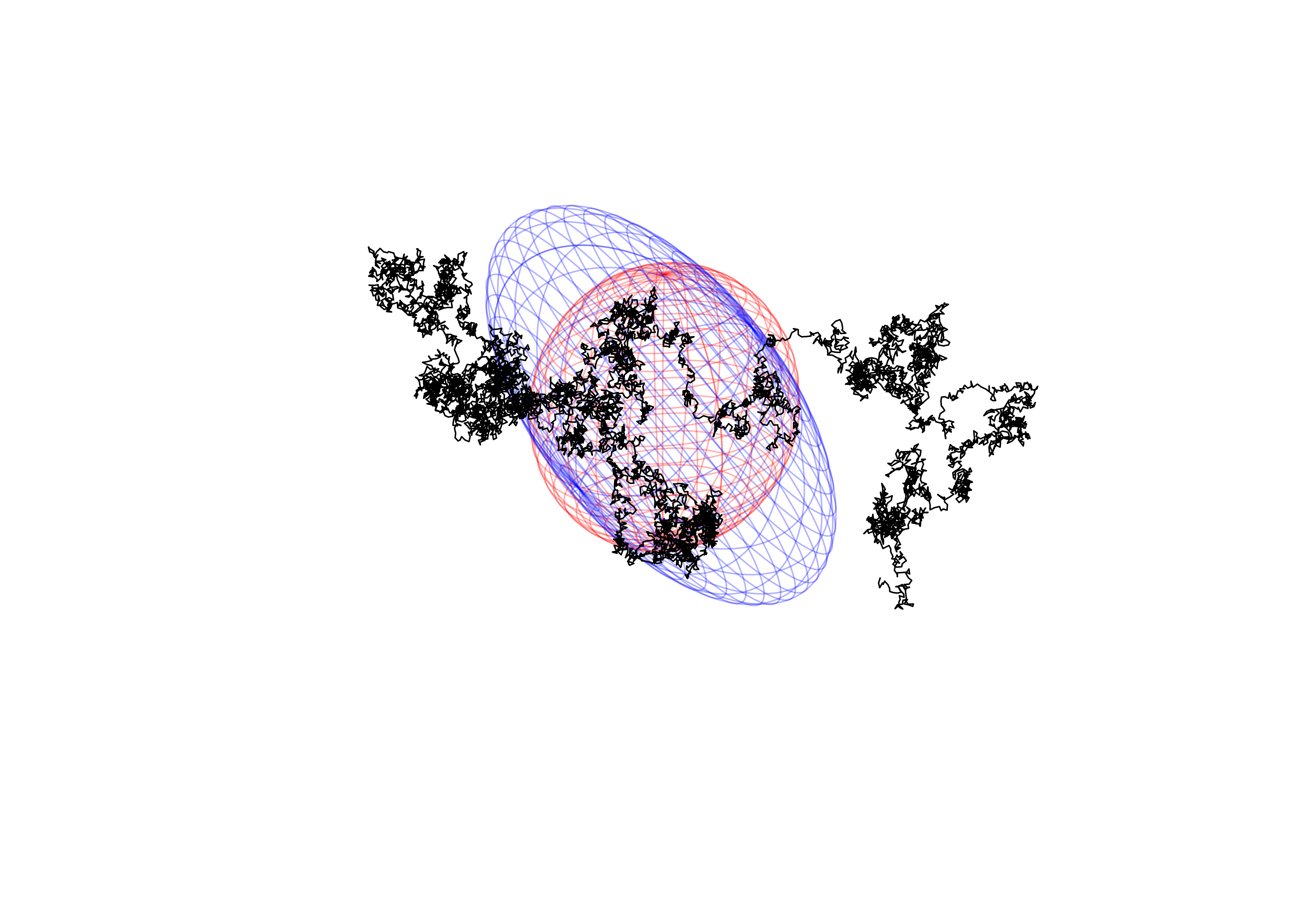
In the following code, a random flight polymer with $N$ segments, each of length $a$, is constructed and displayed. The inertia matrix (actually a tensor) of this polymer can be calculated and diagonalized to find the principal axes. The moment of inertia can be represented as an inertia ellipsoid and this is plotted as a blue wireframe in the code below.

The inertia ellipsoid displayed in blue is that for the polymer at an instant in time. Considering all configurations that the polymer could adopt relative to its centre of mass, one can quantify its size as the radius of gyration, $R_g$: this is the root mean squared distance between all the segments and is also equal to the radius of a hollow sphere with the same moment of inertia as a theoretical random flight polymer. Since for a hollow sphere, $I = \frac{2}{3}mr^2$, the inertia ellipsoid corresponding to the radius of gyration (which is a sphere) can also be displayed (here, in red).

from mpl_toolkits.mplot3d import Axes3D
import matplotlib.pyplot as plt
import numpy as np
import numpy.linalg as linalg

fig = plt.figure()
ax = fig.add_subplot(111, projection='3d')

# Random flight segment length
a = 1.
# Number of random flight segments in the polymer
N = 10000

# pos olds the locations of each segment (Cartesian coordinates)
pos = np.empty((N,3))
pos[0] = (0,0,0)
for i in range(1, N):
    # Pick a new random direction for the next segment uniformly on
    # the unit sphere
    theta = np.arccos(2 * np.random.random() - 1)
    phi = np.random.random() * 2. * np.pi
    # Add on the corresponding displacement vector for this segment.
    dpos = (a * np.sin(theta) * np.cos(phi),
            a * np.sin(theta) * np.sin(phi),
            a * np.cos(theta))
    pos[i] = pos[i-1] + dpos

# Shift the coordinate system to the centre of mass of the polymer
cofm = np.mean(pos, axis=0)
pos -= cofm

# Calculate the moment of interia tensor
mofi = np.empty((3,3))
x, y, z = pos[:,0], pos[:,1], pos[:,2]
Ixx = np.sum(y**2 + z**2)
Iyy = np.sum(x**2 + z**2)
Izz = np.sum(x**2 + y**2)
Ixy = -np.sum(x * y)
Iyz = -np.sum(y * z)
Ixz = -np.sum(x * z)
mofi = np.array(((Ixx, Ixy, Ixz), (Ixy, Iyy, Iyz), (Ixz, Iyz, Izz)))

# Find the rotation matrix and lengths of the semi-principal axes
# by singular value decomposition
U, s, rot = linalg.svd(mofi)
abc = np.sqrt(s/N)
# Rotate the polymer to align with its principal axes
for i,(x,y,z) in enumerate(pos[:]):
    pos[i] = np.dot(np.array((x,y,z)), rot)

# A mesh representing the unit sphere
u = np.linspace(0.0, 2.0 * np.pi, 100)
v = np.linspace(0.0, np.pi, 100)
unit_sphere = np.array((np.outer(np.cos(u), np.sin(v)),
                         np.outer(np.sin(u), np.sin(v)),
                         np.outer(np.ones_like(u), np.cos(v)))).T

# The ellipsoid of inertia
ellipsoid = abc * unit_sphere
ellipsoid = np.dot(ellipsoid, rot)

# The radius of gyration of a theoretical random flight polymer
Rg = np.sqrt(N * a**2 / 6)
# Rg is the radius of a hollow sphere with the same moment of inertia as
# the (theoretical) polymer; the ellipsoid of inertia of this theoretical
# polymer is therefore (2/3) times this radius
sphere = 2 / 3 * Rg * unit_sphere

ax.plot(*pos.T, color="k")
ax.plot_wireframe(*ellipsoid.T,  rstride=4, cstride=4, color='b', alpha=0.3)
ax.plot_wireframe(*sphere.T,  rstride=4, cstride=4, color='r', alpha=0.3)
ax.set_axis_off()
plt.show()

Two different outputs are shown below for two different polymer configurations.