The miscibility of a regular solution
Posted on 12 September 2016
A binary regular solution is one in which the two components, A and B, mix with an entropy of mixing given by the ideal solution model, $$ \Delta_\mathrm{mix}S = -R(x_1\ln x_1 + x_2\ln x_2) $$ but have a non-zero enthalpy of mixing given by the relation $$ \Delta_\mathrm{mix}H = \beta x_1 x_2 $$ where $\beta$ is a parameter describing the difference between the A–B interaction and the average of the A–A and B–B interactions. If $\beta > 0$, there may be some compositions which are immiscible at some temperatures. In this case, it can be shown that there is a maximum temperature, the upper critical solution temperature (UCST), given by $T_\mathrm{c} = \frac{\beta}{2R}$, above which all compositions are miscible.
One way to depict this behaviour is to plot the boundary between the miscible and immiscible regions. This curve can be calculated analytically, but here we deduce it from the position of the minima in $\Delta_\mathrm{mix}G$ as a function of $T$.
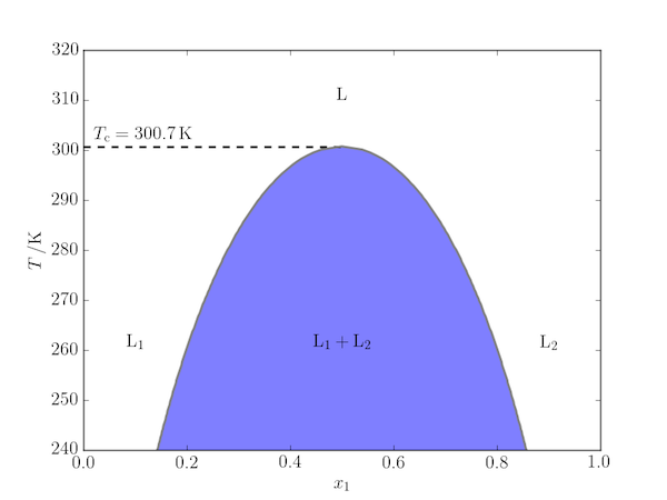
The code used to produce this figure (for $\beta = 5\,\mathrm{kJ\,mol^{-1}}$) is given below. Note that the figure is symmetric about $x_1=\frac{1}{2}$ so we only need to actually calculate the "lefthand" side of it. The immiscible region is highlighted using Matplotlib's fill_between function.
import numpy as np
import matplotlib.pyplot as plt
import matplotlib

# Some matplotlib configuration: make the regular matplotlib font match the
# LaTeX font and increase the font size.
matplotlib.rcParams['mathtext.fontset'] = 'stix'
matplotlib.rcParams['font.family'] = 'STIXGeneral'
matplotlib.rcParams['font.size'] = 16
matplotlib.rcParams['text.usetex'] = True

# The gas constant, J.K-1.mol-1.
R = 8.314

# The regular solution enthalpy of mixing parameter.
beta = 5000

# A grid of mole fraction for component 1. The regular solution model is
# symmetric about x1=x2=0.5, so we only need to calculate its properties from
# 0 to 0.5.
dx = 0.001
x1 = np.arange(dx,0.5,dx)
nx = x1.shape[0]

def get_DG(T, beta, x1):
    """Return the Gibbs free energy of mixing for a regular solution."""

    DG = beta * x1 * (1-x1) + T * R * (x1 * np.log(x1) + (1-x1)*np.log(1-x1))
    return DG

# The upper critical solution temperature (UCST).
Tc = beta / 2 / R
print(Tc)

# A grid of temperatures up to the UCST.
N = 101
Tgrid = np.linspace(240, Tc, N)
# Determine the boundary of miscibility from the position of the minimum
# in Delta-G for x1 = 0 to 0.5 (the "lefthand side" of the free energy plot).
boundary = np.zeros(N)
for i, T in enumerate(Tgrid):
    DG = get_DG(T, beta, x1)
    boundary[i] = x1[np.argmin(DG)]

# Plot a figure: complete the region for x1 > 0.5 as a "reflection" of the
# calculated region.
fig, ax = plt.subplots()
x, y = np.hstack((boundary, 1-boundary[::-1])), np.hstack((Tgrid, Tgrid[::-1]))
ax.plot(x, y, 'gray', lw=2)
ax.fill_between(x, y, alpha=0.5)
ax.set_ylim(240,320)
ax.set_xlim(0,1)
ax.set_xlabel(r'$x_1$')
ax.set_ylabel(r'$T \,/\mathrm{K}$')
ax.text(0.1, 260, r'$\mathrm{L}_1$', ha='center')
ax.text(0.9, 260, r'$\mathrm{L}_2$', ha='center')
ax.text(0.5, 260, r'$\mathrm{L}_1 + \mathrm{L}_2$', ha='center')
ax.text(0.5, 310, r'$\mathrm{L}$', ha='center')
ax.hlines(Tc, 0, 0.5, 'k', linestyles='--', lw=2)
ax.text(0.02, Tc+1, r'$T_\mathrm{{c}} = {:.1f}\,\mathrm{{K}}$'.format(Tc))

plt.show()