The van der Waals equation of state for a gas is: $$ \left(p + \frac{a}{V^2}\right) \left(V - b\right) = RT $$ in terms of the pressure, $p$, molar volume, $V$ and temperature, $T$. $a$ and $b$ are constants which depend on the gas, so it is often useful to recast this equation into reduced form: $$ \left(p_\mathrm{r} + \frac{3}{V_\mathrm{r}^2}\right)\left(V_\mathrm{r}-\frac{1}{3}\right) = \frac{8}{3}T_\mathrm{r}, $$ or equivalently $$ p_\mathrm{r} = \frac{8T_\mathrm{r}}{3V_\mathrm{r}-1} - \frac{3}{V_\mathrm{r}^2}, $$ where the reduced variables $p_\mathrm{r} = p/p_\mathrm{c}$, $V_\mathrm{r} = V/V_\mathrm{c}$ and $T_\mathrm{r} = T / T_\mathrm{c}$ in terms of the critical pressure, volume and temperature: $$ p_\mathrm{c} = \frac{a}{27b^2}, \;\; V_\mathrm{c} = 3b, \;\; k_\mathrm{B}T_\mathrm{c} = \frac{8a}{27b}. $$ Whilst the van der Waals equation does a better job than the ideal gas law of describing the properties of a real gas it suffers from an artefact for $T_\mathrm{r} < 1$ (that is, temperatures $T < T_\mathrm{c}$), as shown in the plot below.

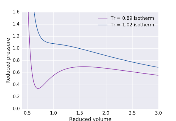
The "loop" in the region between $V_\mathrm{r} \approx 0.6$ and $V_\mathrm{r} \approx 2.5$ is clearly unphysical for it would imply that a gas at a fixed pressure and temperature could have three different equilibrium volumes. In mathematical terms, this region corresponds to values of $p_\mathrm{r}$ where the cubic equation obtained by rearranging the reduced equation of state above, $$ 3p_\mathrm{r}V_\mathrm{r}^3 - (p_\mathrm{r} + 8T_\mathrm{r})V_\mathrm{r}^2 + 9_\mathrm{r} - 3 = 0, $$ has three real roots.

The Maxwell construction deals with this anomaly by recognising that this region corresponds to conditions where the liquid and gas phases coexist: that is, a gas compressed at constant temperature through these volumes will condense with the volume decreasing at constant pressure. Maxwell connected the high and low-volume states with a horizontal line at a fixed pressure such that the areas cut off above and below this line were equal:

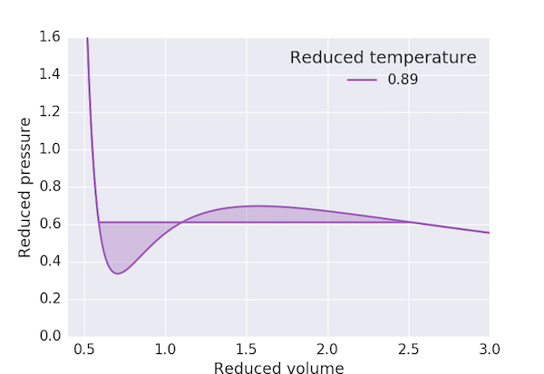
The following program produces a pressure-volume plot for $\mathrm{CO_2}$ using the van der Waals equation of state with the Maxwell construction for $T < T_\mathrm{c}$. We first find the maximum and minimum of the "loop" in $p_\mathrm{r}$ and take our initial guess for the "cut-off" pressure, $p_\mathrm{r,0}$, to be the mean. The three volumes corresponding to this pressure: $V_\mathrm{r,min}$, $V_\mathrm{r,0}$ and $V_\mathrm{r,max}$ are obtained by finding the roots of the above cubic equation. We can then consider the exercise of finding a value of $V_\mathrm{r,0}$ which ensures that the area of the two loops to be the same to be equivalent to finding the solution of the equation $$ \int_{V_\mathrm{r,min}}^{V_\mathrm{r,max}} (p_\mathrm{r} - p_\mathrm{r,0})\,\mathrm{d}V_\mathrm{r} = 0. $$ That is, finding the root of the left hand side: this we can do using Newton's method with scipy.optimize.newton.

import numpy as np
import matplotlib.pyplot as plt
from scipy.integrate import quad
from scipy.optimize import newton
from scipy.signal import argrelextrema

palette = iter(['#9b59b6', '#4c72b0', '#55a868', '#c44e52', '#dbc256'])

# Critical pressure, volume and temperature
# These values are for the van der Waals equation of state for CO2:
# (p - a/V^2)(V-b) = RT. Units: p is in Pa, Vc in m3/mol and T in K.
pc = 7.404e6
Vc = 1.28e-4
Tc = 304

def vdw(Tr, Vr):
    """Van der Waals equation of state.

    Return the reduced pressure from the reduced temperature and volume.

    """

    pr = 8*Tr/(3*Vr-1) - 3/Vr**2
    return pr


def vdw_maxwell(Tr, Vr):
    """Van der Waals equation of state with Maxwell construction.

    Return the reduced pressure from the reduced temperature and volume,
    applying the Maxwell construction correction to the unphysical region
    if necessary.

    """

    pr = vdw(Tr, Vr)
    if Tr >= 1:
        # No unphysical region above the critical temperature.
        return pr

    if min(pr) < 0:
         raise ValueError('Negative pressure results from van der Waals'
                         ' equation of state with Tr = {} K.'.format(Tr))

    # Initial guess for the position of the Maxwell construction line:
    # the volume corresponding to the mean pressure between the minimum and
    # maximum in reduced pressure, pr.
    iprmin = argrelextrema(pr, np.less)
    iprmax = argrelextrema(pr, np.greater)
    Vr0 = np.mean([Vr[iprmin], Vr[iprmax]])

    def get_Vlims(pr0):
        """Solve the inverted van der Waals equation for reduced volume.

        Return the lowest and highest reduced volumes such that the reduced
        pressure is pr0. It only makes sense to call this function for
        T<Tc, ie below the critical temperature where there are three roots.

        """

        eos = np.poly1d( (3*pr0, -(pr0+8*Tr), 9, -3) )
        roots = eos.r
        roots.sort()
        Vrmin, _, Vrmax = roots
        return Vrmin, Vrmax

    def get_area_difference(Vr0):
        """Return the difference in areas of the van der Waals loops.

        Return the difference between the areas of the loops from Vr0 to Vrmax
        and from Vrmin to Vr0 where the reduced pressure from the van der Waals
        equation is the same at Vrmin, Vr0 and Vrmax. This difference is zero
        when the straight line joining Vrmin and Vrmax at pr0 is the Maxwell
        construction.

        """

        pr0 = vdw(Tr, Vr0)
        Vrmin, Vrmax = get_Vlims(pr0)
        return quad(lambda vr: vdw(Tr, vr) - pr0, Vrmin, Vrmax)[0]

    # Root finding by Newton's method determines Vr0 corresponding to
    # equal loop areas for the Maxwell construction.
    Vr0 = newton(get_area_difference, Vr0)
    pr0 = vdw(Tr, Vr0)
    Vrmin, Vrmax = get_Vlims(pr0)

    # Set the pressure in the Maxwell construction region to constant pr0.
    pr[(Vr >= Vrmin) & (Vr <= Vrmax)] = pr0
    return pr

Vr = np.linspace(0.5, 3, 500)

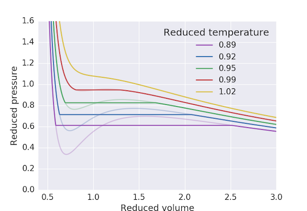
def plot_pV(T):
    Tr = T / Tc
    c = next(palette)
    ax.plot(Vr, vdw(Tr, Vr), lw=2, alpha=0.3, color=c)
    ax.plot(Vr, vdw_maxwell(Tr, Vr), lw=2, color=c, label='{:.2f}'.format(Tr))

fig, ax = plt.subplots()

for T in range(270, 320, 10):
    plot_pV(T)

ax.set_xlim(0.4, 3)
ax.set_xlabel('Reduced volume')
ax.set_ylim(0, 1.6)
ax.set_ylabel('Reduced pressure')
ax.legend(title='Reduced temperature')

plt.show()