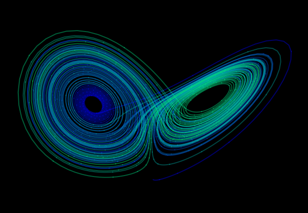
The Lorenz system of coupled, ordinary, first-order differential equations have chaotic solutions for certain parameter values $\sigma$, $\rho$ and $\beta$ and initial conditions, $u(0)$, $v(0)$ and $w(0)$.

$$ \begin{align*} \frac{\mathrm{d}u}{\mathrm{d}t} &= \sigma (v - u)\\ \frac{\mathrm{d}v}{\mathrm{d}t} &= \rho u - v - uw\\ \frac{\mathrm{d}w}{\mathrm{d}t} &= uv - \beta w \end{align*} $$

The following program plots the Lorenz attractor (the values of $x$, $y$ and $z$ as a parametric function of time) on a Matplotlib 3D projection.

This code is also available on my GitHub page.

import numpy as np
from scipy.integrate import solve_ivp
import matplotlib.pyplot as plt
from mpl_toolkits.mplot3d import Axes3D

# Create an image of the Lorenz attractor.
# The maths behind this code is described in the scipython blog article
# at https://scipython.com/blog/the-lorenz-attractor/
# Christian Hill, January 2016.
# Updated, January 2021 to use scipy.integrate.solve_ivp.

WIDTH, HEIGHT, DPI = 1000, 750, 100

# Lorenz paramters and initial conditions.
sigma, beta, rho = 10, 2.667, 28
u0, v0, w0 = 0, 1, 1.05

# Maximum time point and total number of time points.
tmax, n = 100, 10000

def lorenz(t, X, sigma, beta, rho):
    """The Lorenz equations."""
    u, v, w = X
    up = -sigma*(u - v)
    vp = rho*u - v - u*w
    wp = -beta*w + u*v
    return up, vp, wp

# Integrate the Lorenz equations.
soln = solve_ivp(lorenz, (0, tmax), (u0, v0, w0), args=(sigma, beta, rho),
                 dense_output=True)
# Interpolate solution onto the time grid, t.
t = np.linspace(0, tmax, n)
x, y, z = soln.sol(t)

# Plot the Lorenz attractor using a Matplotlib 3D projection.
fig = plt.figure(facecolor='k', figsize=(WIDTH/DPI, HEIGHT/DPI))
ax = fig.gca(projection='3d')
ax.set_facecolor('k')
fig.subplots_adjust(left=0, right=1, bottom=0, top=1)

# Make the line multi-coloured by plotting it in segments of length s which
# change in colour across the whole time series.
s = 10
cmap = plt.cm.winter
for i in range(0,n-s,s):
    ax.plot(x[i:i+s+1], y[i:i+s+1], z[i:i+s+1], color=cmap(i/n), alpha=0.4)

# Remove all the axis clutter, leaving just the curve.
ax.set_axis_off()

plt.savefig('lorenz.png', dpi=DPI)
plt.show()