The Klein–Nishina formula

The Klein–Nishina formula gives the differential cross section for the scattering of photons off an electron. At low energies, light scatters elastically (Thomson scattering); at higher energies (for example, gamma radiation), inelastic Compton scattering occurs. In terms of the incoming and outgoing photon wavelengths, $\lambda$ and $\lambda'$:

$$ \frac{\mathrm{d}\sigma}{\mathrm{d}\Omega} = \frac{\hbar^2\alpha^2}{2m_e^2c^2}\left(\frac{\lambda}{\lambda'}\right)^2\left[\frac{\lambda}{\lambda'} + \frac{\lambda'}{\lambda} - \sin^2\theta\right], $$

where $\mathrm{d}\sigma$ is the cross section for scattering into solid angle $\mathrm{d}\Omega$ at an angle $\theta$ from the incoming direction. The scattered wavelength is given by the Compton scattering formula:

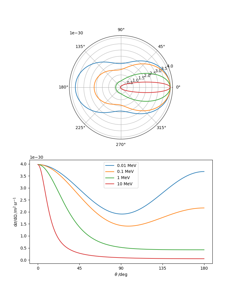
The Python code below plots the following figure for the angular dependence of the differential cross section at different incoming photon energies. At low energies, forward and back-scattering are equally likely (blue line: 10 keV); at high energies, forward scattering dominates and most of the photon's energy is transferred to the electron (red line: 10 MeV).

import numpy as np
import matplotlib.pyplot as plt
from scipy.constants import e, h, hbar, alpha, c, m_e
DPI = 100

# A bunch of constants factored into a single variable.
f = (hbar * alpha / m_e / c)**2 / 2
# A grid of scattering angles in rad.
theta = np.arange(0, 2*np.pi, 0.01)
n = len(theta)


def plot_diff_xsec(E):
    """Plot the differential cross section for incoming photon energy, E."""

    # Incoming photon frequency (s-1) and wavelength (m).
    nu = E * 1.e6 * e / h
    lam = c / nu

    # Scattered photon wavelength (m).
    lamp = lam + h / m_e / c * (1 - np.cos(theta))
    P = lam / lamp
    # Differential cross section given by the Klein-Nishina formula.
    dsigma_dOmega = f * P**2 * (P + 1/P - np.sin(theta)**2)

    # Plot the polar and Cartesian plots.
    ax1.plot(theta, dsigma_dOmega, label=str(E) + r' MeV')
    # Because of the symmetry, we only really need angles 0 -> 180 deg.
    ax2.plot(np.degrees(theta[:n//2]), dsigma_dOmega[:n//2],
             label=str(E) + r' MeV')

# A Matplotlib figure with a polar Axes above a Cartesian one.
fig = plt.figure(figsize=(800/DPI, 1000/DPI))
ax1 = fig.add_subplot(211, projection='polar')
ax2 = fig.add_subplot(212)

# Our grid of photon energies (in MeV).
Egrid = 0.01, 0.1, 1, 10
for E in Egrid:
    plot_diff_xsec(E)
ax2.set_xlabel(r'$\theta\;/\mathrm{deg}$')
ax2.set_ylabel(r'$\mathrm{d}\sigma/\mathrm{d}\Omega\;/\mathrm{m^2\,sr^{-1}}$')
# Set the Cartesian x-axis ticks to sensible values (in degrees).
ax2.set_xticks([0, 45, 90, 135, 180])

plt.legend()
plt.show()

Comments

Comments are pre-moderated. Please be patient and your comment will appear soon.

Skyler 1 year, 11 months ago

Exactly what I was looking for, and very digestibly presented.

Thank you

Link | Reply

The Klein–Nishina formula

Posted by: christian on 18 Dec 2021

Comments

Skyler 1 year, 11 months ago

New Comment