The hanging chain: part 2

Posted by: christian on 28 Feb 2018

(0 comments)

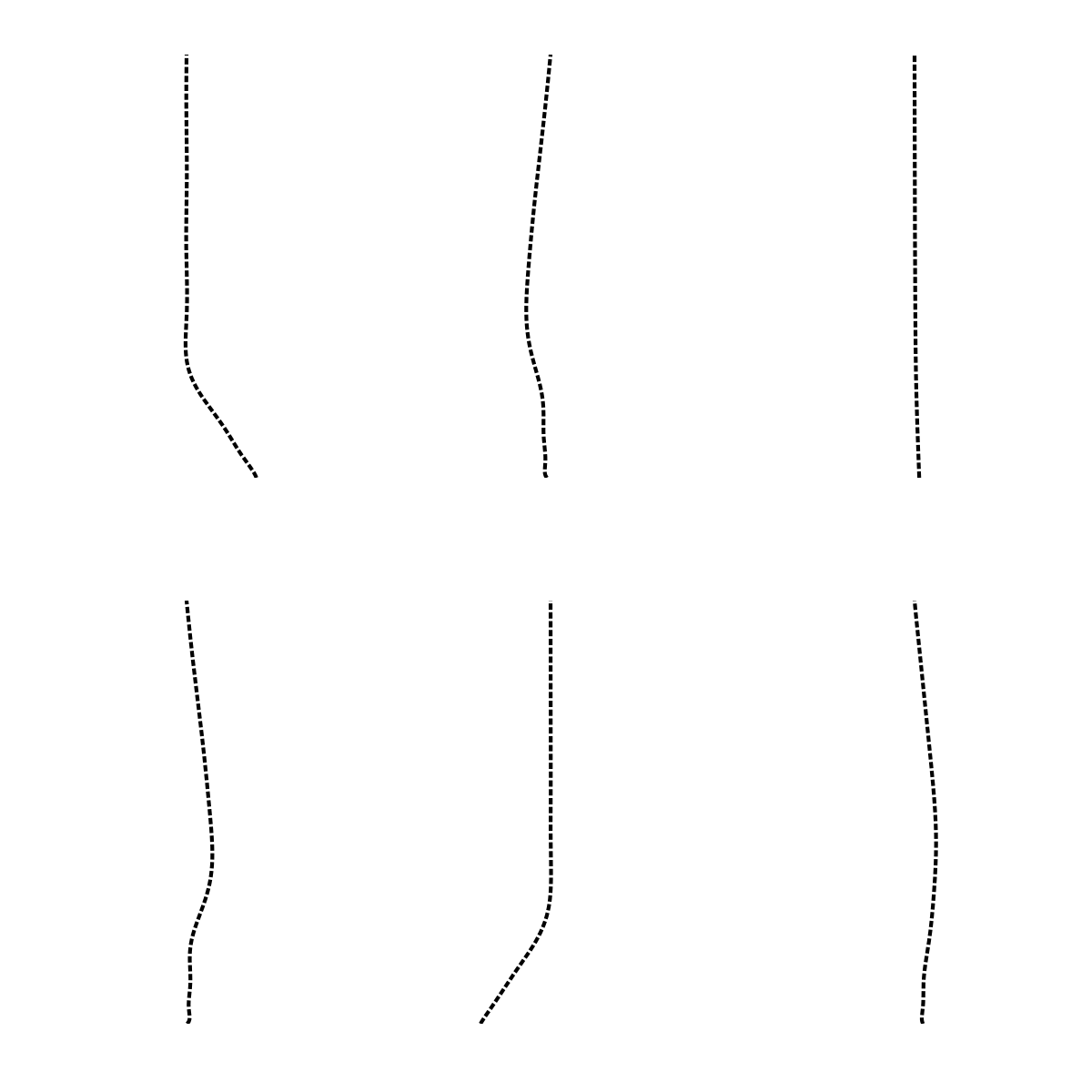
The previous blog post described the normal modes of a chain swinging under its own weight. Here we describe the motion of a chain after an arbitrary displacement as a linear combination of such normal modes.

The code for this project is on my github page and the Jupyter Notebook can be run in nbviewer here.

Using the same notation as before, suppose the state of the chain at $t=0$ can be described as $x(z,0) = f(z)$. The general solution to the Bessel differential equation derived previously must involve a linear combination of the modes: $$ x(z,t) = \sum_{n=1}^\infty J_0\left(2\omega_n\sqrt{z/g}\right)A_n\cos(\omega_n t), $$ where we again assume that the chain is initially not moving so there is no sine term. The coefficients $A_n$ may be determined as follows. At $t=0$, in terms of our scaled coordinate, $u = 2\sqrt{z/g}$, $$ \sum_{n=1}^\infty J\left(\omega_n u\right)A_n = f(u). $$ The Bessel functions $J_0(\omega_n u)$ are orthogonal on $(0,1)$ with respect to the weight function $u$: $$ \int_0^1 u J_0(\omega_n u)J_0(\omega_m u)\,\mathrm{d}u = \frac{1}{2}\delta_{nm}[J_1(\omega_n)]^2, $$ where $\delta_{nm}$ is the Kronecker delta. The coefficients, $A_n$ can therefore be obtained by projecting the function $f(u)$ onto the Bessel functions $J_0(\omega_n u)$. With a suitable scaling to the interval on $u$ of $(0, b)$ (where $b = 2\sqrt{L/g}$ corresponds to $z=L$) instead of $(0,1)$, one obtains $$ A_n = \frac{2\int_0^b u f(u) J_0(\omega_n u / b)\,\mathrm{d}u}{\left[ b J_1(\omega_n) \right]^2}. $$ These are the coefficients to the Fourier–Bessel series expansion of $f(u)$.

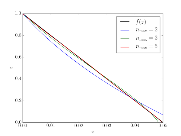
For example, consider the linear function $f(z) = pz + q$ where $f(0)=d$: this would correspond to displacing the end of the chain horizontally through a distance $d$ whilst keeping the chain taut. We have $q=d$ and $p=-d/L$. The series expansion, truncated at $n=2$, 3, and 5 terms, is illustrated below.

import numpy as np
from scipy.special import j0, j1, jn_zeros
from scipy.integrate import quad
from matplotlib import rc
import matplotlib.pyplot as plt

# Use LaTeX throughout the figure for consistency
rc('font', **{'family': 'serif', 'serif': ['Computer Modern'], 'size': 16})
rc('text', usetex=True)

# Acceleration due to gravity, m.s-2
g = 9.81
# Chain length, m
L = 1
# Vertical axis (m)
N = 201
z = np.linspace(0, L, N)
# Scaled vertical axis
u = 2 * np.sqrt(z/g)

# The exact function of z, x(z,0): linear from (0,d) to (L,0):
d, c = 0.05, L
p, q = -d/c, d
def f(u):
    z = u**2 * g / 4
    return p*z + q

nmax = 10
# jn_zeros calculates the first n zeros of the zero-th order Bessel function
# of the first kind
w = jn_zeros(0, nmax)
b = 2 * np.sqrt(L/g)

def func(u, n):
    """The integrand for the Fourier-Bessel coefficient A_n."""
    return u * f(u) * j0(w[n-1] / b * u)

# Calculate the Fourier-Bessel coefficients using numerical integration
A = []
for n in range(1, nmax+1):
    An = quad(func, 0, b, args=(n,))[0] * 2 / (b * j1(w[n-1]))**2
    A.append(An)

# Create a labelled plot comparing f(z) with the Fourier-Bessel series
# approximation truncated at 2, 3 and 5 terms.
plt.plot(f(u), z, 'k', lw=2, label='$f(z)$')
for nmax in (2,3,5):
    ffit = np.zeros(N)
    for n in range(nmax):
        ffit += A[n-1] * j0(w[n-1] / b * u)
    plt.plot(ffit, z, label=r'$n_\mathrm{max} = '+'{}$'.format(nmax))
plt.xlim(0,d)
plt.xlabel(r'$x$')
plt.ylabel(r'$z$')
plt.legend()

plt.savefig('fourier_bessel.png')
plt.show()

In this case, convergence is relatively quick:

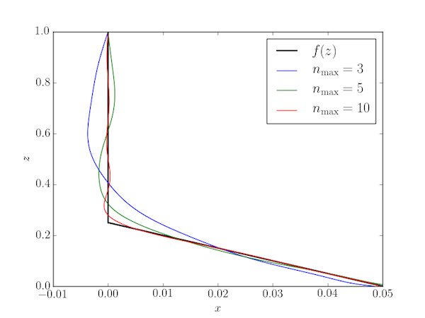
A slightly different initial condition displaces only the lower portion of the chain for $z>c$ where $0<c<L$:

# The exact function of z, x(z,0): linear from (0,d) to (c,0) then zero
# from (c,0) to (L,0).
d, c = 0.05, L/4
p, q = -d/c, d
def f(u):
    z = u**2 * g / 4
    # We have to cater z as a scalar and as an array since u could be passed as
    # either and we want to use boolean indexing to set h = 0 for z > c.
    if np.isscalar(z):
        if z > c:
            return 0
        return p*z + q
    h = p*z + q
    h[z>c] = 0
    return h

Convergence is slightly slower in this case:

• ← The hanging chain
• Bertrand's Paradox →