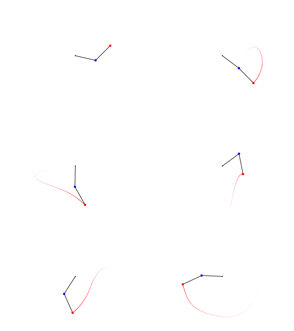
In classical mechanics, a double pendulum is a pendulum attached to the end of another pendulum. Its equations of motion are often written using the Lagrangian formulation of mechanics and solved numerically, which is the approach taken here. The dynamics of the double pendulum are chaotic and complex, as illustrated below.

The code:

import sys
import numpy as np
from scipy.integrate import odeint
import matplotlib.pyplot as plt
from matplotlib.patches import Circle

# Pendulum rod lengths (m), bob masses (kg).
L1, L2 = 1, 1
m1, m2 = 1, 1
# The gravitational acceleration (m.s-2).
g = 9.81

def deriv(y, t, L1, L2, m1, m2):
    """Return the first derivatives of y = theta1, z1, theta2, z2."""
    theta1, z1, theta2, z2 = y

    c, s = np.cos(theta1-theta2), np.sin(theta1-theta2)

    theta1dot = z1
    z1dot = (m2*g*np.sin(theta2)*c - m2*s*(L1*z1**2*c + L2*z2**2) -
             (m1+m2)*g*np.sin(theta1)) / L1 / (m1 + m2*s**2)
    theta2dot = z2
    z2dot = ((m1+m2)*(L1*z1**2*s - g*np.sin(theta2) + g*np.sin(theta1)*c) + 
             m2*L2*z2**2*s*c) / L2 / (m1 + m2*s**2)
    return theta1dot, z1dot, theta2dot, z2dot

def calc_E(y):
    """Return the total energy of the system."""

    th1, th1d, th2, th2d = y.T
    V = -(m1+m2)*L1*g*np.cos(th1) - m2*L2*g*np.cos(th2)
    T = 0.5*m1*(L1*th1d)**2 + 0.5*m2*((L1*th1d)**2 + (L2*th2d)**2 +
            2*L1*L2*th1d*th2d*np.cos(th1-th2))
    return T + V

# Maximum time, time point spacings and the time grid (all in s).
tmax, dt = 30, 0.01
t = np.arange(0, tmax+dt, dt)
# Initial conditions: theta1, dtheta1/dt, theta2, dtheta2/dt.
y0 = np.array([3*np.pi/7, 0, 3*np.pi/4, 0])

# Do the numerical integration of the equations of motion
y = odeint(deriv, y0, t, args=(L1, L2, m1, m2))

# Check that the calculation conserves total energy to within some tolerance.
EDRIFT = 0.05
# Total energy from the initial conditions
E = calc_E(y0)
if np.max(np.sum(np.abs(calc_E(y) - E))) > EDRIFT:
    sys.exit('Maximum energy drift of {} exceeded.'.format(EDRIFT))

# Unpack z and theta as a function of time
theta1, theta2 = y[:,0], y[:,2]

# Convert to Cartesian coordinates of the two bob positions.
x1 = L1 * np.sin(theta1)
y1 = -L1 * np.cos(theta1)
x2 = x1 + L2 * np.sin(theta2)
y2 = y1 - L2 * np.cos(theta2)

# Plotted bob circle radius
r = 0.05
# Plot a trail of the m2 bob's position for the last trail_secs seconds.
trail_secs = 1
# This corresponds to max_trail time points.
max_trail = int(trail_secs / dt)

def make_plot(i):
    # Plot and save an image of the double pendulum configuration for time
    # point i.
    # The pendulum rods.
    ax.plot([0, x1[i], x2[i]], [0, y1[i], y2[i]], lw=2, c='k')
    # Circles representing the anchor point of rod 1, and bobs 1 and 2.
    c0 = Circle((0, 0), r/2, fc='k', zorder=10)
    c1 = Circle((x1[i], y1[i]), r, fc='b', ec='b', zorder=10)
    c2 = Circle((x2[i], y2[i]), r, fc='r', ec='r', zorder=10)
    ax.add_patch(c0)
    ax.add_patch(c1)
    ax.add_patch(c2)

    # The trail will be divided into ns segments and plotted as a fading line.
    ns = 20
    s = max_trail // ns

    for j in range(ns):
        imin = i - (ns-j)*s
        if imin < 0:
            continue
        imax = imin + s + 1
        # The fading looks better if we square the fractional length along the
        # trail.
        alpha = (j/ns)**2
        ax.plot(x2[imin:imax], y2[imin:imax], c='r', solid_capstyle='butt',
                lw=2, alpha=alpha)

    # Centre the image on the fixed anchor point, and ensure the axes are equal
    ax.set_xlim(-L1-L2-r, L1+L2+r)
    ax.set_ylim(-L1-L2-r, L1+L2+r)
    ax.set_aspect('equal', adjustable='box')
    plt.axis('off')
    plt.savefig('frames/_img{:04d}.png'.format(i//di), dpi=72)
    plt.cla()


# Make an image every di time points, corresponding to a frame rate of fps
# frames per second.
# Frame rate, s-1
fps = 10
di = int(1/fps/dt)
fig = plt.figure(figsize=(8.3333, 6.25), dpi=72)
ax = fig.add_subplot(111)

for i in range(0, t.size, di):
    print(i // di, '/', t.size // di)
    make_plot(i)

The images are saved to a subdirectory, frames/ and can be converted into an animated gif, for example with ImageMagick's convert utility.

Derivation of the equations of motion

The derivation of the double pendulum equations of motion using the Lagrangian formulation has become a standard exercise in introductory classical mechanics, but an outline is given below. There are many, many similar derivations on the internet. We use the following coordinate system:

The two degrees of freedom are taken to be $\theta_1$ and $\theta_2$, the angle of each pendulum rod from the vertical. The components of the bob positions and velocities are

$$ \begin{align*} x_1 & = l_1\sin\theta_1 & \dot{x}_1 &= l_1\dot{\theta}_1\cos\theta_1\\ y_1 & = -l_1\cos\theta_1 & \dot{y}_1 &= l_1\dot{\theta}_1\sin\theta_1\\ x_2 & = l_1\sin\theta_1 + l_2\sin\theta_2 & \dot{x}_2 &= l_1\dot{\theta}_1\cos\theta_1 + l_2\dot{\theta}_2\cos\theta_2\\ y_2 & = -l_1\cos\theta_1 - l_2\cos\theta_2 & \dot{y}_2 &= l_1\dot{\theta}_1\sin\theta_1 + l_2\dot{\theta}_2\sin\theta_2 \end{align*} $$

The potential and kinetic energies are then

$$ \begin{align*} V &= m_1gy_1 + m_2gy_2 = -(m_1 + m_2)l_1g\cos\theta_1 - m_2l_2g\cos\theta_2\\ T &= \tfrac{1}{2}m_1v_1^2 + \tfrac{1}{2}m_2v_2^2 = \tfrac{1}{2}m_1(\dot{x}_1^2 + \dot{y}_1^2) + \tfrac{1}{2}m_2(\dot{x}_2^2 + \dot{y}_2^2)\\ &= \tfrac{1}{2}m_1l_1^2\dot{\theta}_1^2 + \tfrac{1}{2}m_2[l_1^2\dot{\theta}_1^2 + l_2^2\dot{\theta}_2^2 + 2l_1l_2\dot{\theta}_1\dot{\theta}_2\cos(\theta_1 - \theta_2)] \end{align*} $$

The Lagrangian, $\mathcal{L} = T - V$ is therefore:

$$ \begin{align*} \mathcal{L} = \tfrac{1}{2}(m_1+m_2)l_1^2\dot{\theta}_1^2 + \tfrac{1}{2}m_2l_2^2\dot{\theta}_2^2 + m_2l_1l_2\dot{\theta}_1\dot{\theta}_2\cos(\theta_1 - \theta_2) + (m_1+m_2)l_1g\cos\theta_1 + m_2gl_2\cos\theta_2. \end{align*} $$

The Euler-Lagrange equations are:

$$ \begin{align*} \frac{\mathrm{d}}{\mathrm{d}t}\left(\frac{\partial\mathcal{L}}{\partial \dot{q}_i}\right) - \frac{\partial \mathcal{L}}{\partial q_i} = 0 \quad \mathrm{for}\;q_i = \theta_1, \theta_2. \end{align*} $$

For these coordinates, after some calculus and algebra, we get:

$$ \begin{align*} (m_1 + m_2)l_1 \ddot{\theta}_1 + m_2l_2\ddot{\theta}_2\cos(\theta_1 - \theta_2) + m_2l_2\dot{\theta}_2^2\sin(\theta_1 - \theta_2) + (m_1+m_2)g\sin\theta_1 &= 0,\\ m_2l_2\ddot{\theta}_2 + m_2l_1\ddot{\theta}_1\cos(\theta_1 - \theta_2) - m_2l_1\dot{\theta}_1^2\sin(\theta_1 - \theta_2) + m_2g\sin\theta_2 = 0. \end{align*} $$

scipy's ordinary differential equation solver, integrate.odeint needs to work with systems of first-order differential equations, so let $z_1 \equiv \dot{\theta_1} \Rightarrow \ddot{\theta}_1 = \dot{z}_1$ and $z_2 \equiv \dot{\theta_2} \Rightarrow \ddot{\theta}_2 = \dot{z}_2$. After some rearranging, the following expressions for $\dot{z}_1$ and $\dot{z}_2$ are obtained:

$$ \begin{align*} \dot{z}_1 = \frac{m_2g\sin\theta_2\cos(\theta_1-\theta_2) - m_2\sin(\theta_1 - \theta_2)[l_1z_1^2\cos(\theta_1 - \theta_2) + l_2z_2^2] - (m_1+m_2)g\sin\theta_1}{l_1[m_1 + m_2\sin^2(\theta_1-\theta_2)]},\\ \dot{z}_2 = \frac{(m_1+m_2)[l_1z_1^2\sin(\theta_1-\theta_2) - g\sin\theta_2 + g\sin\theta_1\cos(\theta_1-\theta_2)]+m_2l_2z_2^2\sin(\theta_1-\theta_2)\cos(\theta_1-\theta_2)}{l_2[m_1 + m_2\sin^2(\theta_1-\theta_2)]} \end{align*} $$

It is these equations which appear in the function deriv in the code above.