The Debye length
Posted on 21 August 2018
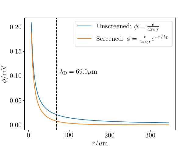
An important concept in plasma physics is the Debye length, which describes the screening of a charge's electrostatic potential due to the net effect of the interactions it undergoes with the other mobile charges (electrons and ions) in the system. It can be shown that, given a set of reasonable assumptions about the behaviour of charges in the plasma, the electric potential due to a "test charge", $q_\mathrm{T}$ is given by $$ \phi = \frac{q_\mathrm{T}}{4\pi\epsilon_0 r}\exp\left(-\frac{r}{\lambda_\mathrm{D}}\right), $$ where the electron Debye length, $$ \lambda_\mathrm{D} = \sqrt{\frac{\epsilon_0 T_e}{e^2n_0}}, $$ for an electron temperature $T_e$ expressed as an energy (i.e. $T_e = k_\mathrm{B}T_e'$ where $T_e'$ is in K) and number density $n_0$. Rigorous derivations, starting from Gauss' Law and solving the resulting Poisson equation with a Green's function are given elsewhere (e.g. Section 7.2.2. in J. P. Freidberg, Plasma Physics and Fusion Energy, CUP (2008)).
The following Python code plots the shielded and unshielded Coulomb potential due to a point test charge $q_\mathrm{T} = +e$, assuming an electron temperature and density typical of a tokamak magnetic confinement nuclear fusion device.
import numpy as np
from scipy.constants import k as kB, epsilon_0, e
from matplotlib import rc
import matplotlib.pyplot as plt

rc('font', **{'family': 'serif', 'serif': ['Computer Modern'], 'size': 16})
rc('text', usetex=True)
# We need the following so that the legend labels are vertically centred on
# their indicator lines.
rc('text.latex', preview=True)

def calc_debye_length(Te, n0):
    """Return the Debye length for a plasma characterised by Te, n0.

    The electron temperature Te should be given in eV and density, n0
    in cm-3. The debye length is returned in m.

    """

    return np.sqrt(epsilon_0 * Te / e / n0 / 1.e-6)

def calc_unscreened_potential(r, qT):
   return qT * e / 4 / np.pi / epsilon_0 / r
def calc_e_potential(r, lam_De, qT):
    return calc_unscreened_potential(r, qT) * np.exp(-r / lam_De)

# plasma electron temperature (eV) and density (cm-3) for a typical tokamak.
Te, n0 = 1.e8 * kB / e, 1.e26
lam_De = calc_debye_length(Te, n0)
print(lam_De)

# range of distances to plot phi for, in m.
rmin = lam_De / 10
rmax = lam_De * 5
r = np.linspace(rmin, rmax, 100)
qT = 1
phi_unscreened = calc_unscreened_potential(r, qT)
phi = calc_e_potential(r, lam_De, qT)

# Plot the figure. Apologies for the ugly and repetitive unit conversions from
# m to µm and from V to mV.
fig, ax = plt.subplots()
ax.plot(r*1.e6, phi_unscreened * 1000,
                label=r'Unscreened: $\phi = \frac{e}{4\pi\epsilon_0 r}$')
ax.plot(r*1.e6, phi * 1000,
                label=r'Screened: $\phi = \frac{e}{4\pi\epsilon_0 r}'
                      r'e^{-r/\lambda_\mathrm{D}}$')
ax.axvline(lam_De*1.e6, ls='--', c='k')
ax.annotate(xy=(lam_De*1.1*1.e6, max(phi_unscreened)/2 * 1000),
            s=r'$\lambda_\mathrm{D} = %.1f \mathrm{\mu m}$' % (lam_De*1.e6))
ax.legend()
ax.set_xlabel(r'$r/\mathrm{\mu m}$')
ax.set_ylabel(r'$\phi/\mathrm{mV}$')
plt.savefig('debye_length.png')
plt.show()