Simulating the Belousov-Zhabotinsky reaction

Posted by: christian on 27 Jul 2017

(0 comments)

The Belousov-Zhabotinsky (BZ) reaction is a classical example of a non-equibrium chemical oscillator in which the components exhibit periodic changes in concentration.

The model

The BZ reaction mechanism is complex and still not fully understood, but its essential features can be captured in a simple reaction model involving three chemical substrates[1, 2]:

where $\alpha$, $\beta$ and $\gamma$ are rate constants. The concentrations of $\mathrm{A}$, $\mathrm{B}$ and $\mathrm{C}$ may be followed on a grid of discrete time points through the equations

In order to account for the spatial variation in concentration the reaction is assumed to take place on a discrete two-dimensional grid of cells. At every time step the concentration of each component at a cell is set to its average across that cell and its eight neighbours (the Moore neighbourhood). The grid is wrapped top-to-bottom and left-to-right and, for simplicity, the concentrations are constrained to lie between 0 and 1. The initial concentrations are set to random values in this range.

Example outputs

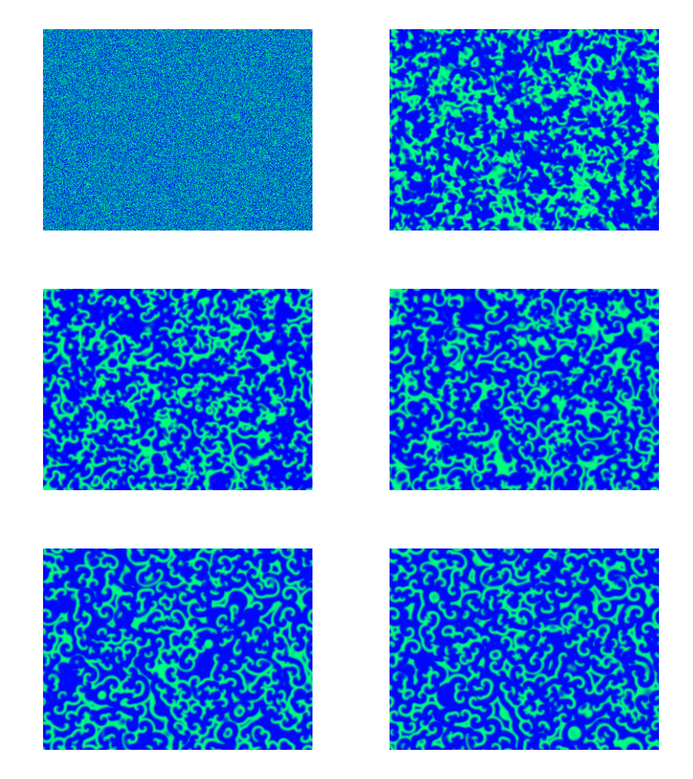
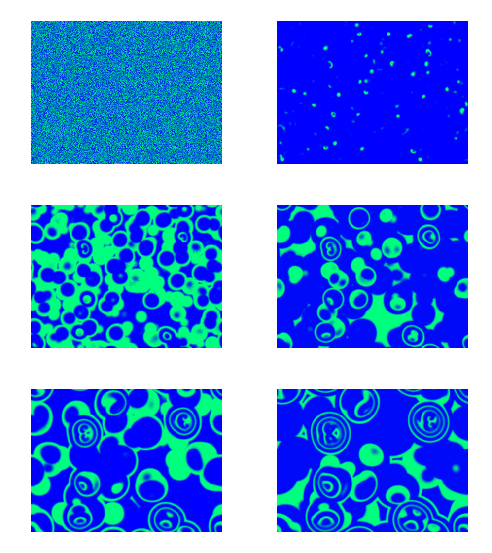
Spirals and waves appear spontaneously and unpredictably in the concentration profiles of the reaction components on a scale dictated by the values of $\alpha$, $\beta$ and $\gamma$.

For $\alpha=\beta=\gamma=1$:

For $\alpha=1.2, \beta=\gamma=1$:

The code

The Python code below creates an animation of the BZ reaction using NumPy and Matplotlib. Significant speed improvements over Python looping are achieved by averaging the neighbour concentrations by convolution with a $3\times 3$ array of values $\frac{1}{9}$ (see scipy.signal.convolve2d).

To create the animation movie, ffmpeg or some other encoder should be installed.

import numpy as np
from scipy.signal import convolve2d
import matplotlib.pyplot as plt
from matplotlib import animation

# Width, height of the image.
nx, ny = 600, 450
# Reaction parameters.
alpha, beta, gamma = 1, 1, 1

def update(p,arr):
    """Update arr[p] to arr[q] by evolving in time."""

    # Count the average amount of each species in the 9 cells around each cell
    # by convolution with the 3x3 array m.
    q = (p+1) % 2
    s = np.zeros((3, ny,nx))
    m = np.ones((3,3)) / 9
    for k in range(3):
        s[k] = convolve2d(arr[p,k], m, mode='same', boundary='wrap')
    # Apply the reaction equations
    arr[q,0] = s[0] + s[0]*(alpha*s[1] - gamma*s[2])
    arr[q,1] = s[1] + s[1]*(beta*s[2] - alpha*s[0])
    arr[q,2] = s[2] + s[2]*(gamma*s[0] - beta*s[1])
    # Ensure the species concentrations are kept within [0,1].
    np.clip(arr[q], 0, 1, arr[q])
    return arr

# Initialize the array with random amounts of A, B and C.
arr = np.random.random(size=(2, 3, ny, nx))

# Set up the image
fig, ax = plt.subplots()
im = ax.imshow(arr[0,0], cmap=plt.cm.winter)
ax.axis('off')

def animate(i, arr):
    """Update the image for iteration i of the Matplotlib animation."""

    arr = update(i % 2, arr)
    im.set_array(arr[i % 2, 0])
    return [im]

anim = animation.FuncAnimation(fig, animate, frames=200, interval=5,
                               blit=False, fargs=(arr,))

# To view the animation, uncomment this line
plt.show()

# To save the animation as an MP4 movie, uncomment this line
#anim.save(filename='bz.mp4', fps=30)

References

1. P. Ball, "Designing the Molecular World: Chemistry at the Frontier", Princeton (1994)
2. A. Turner, "A simple model of the Belousov-Zhabotinsky reaction from first principles", Implementation note, UCL, (2009).

• ← The harmonically-driven pendulum
• Evolution of a free particle →