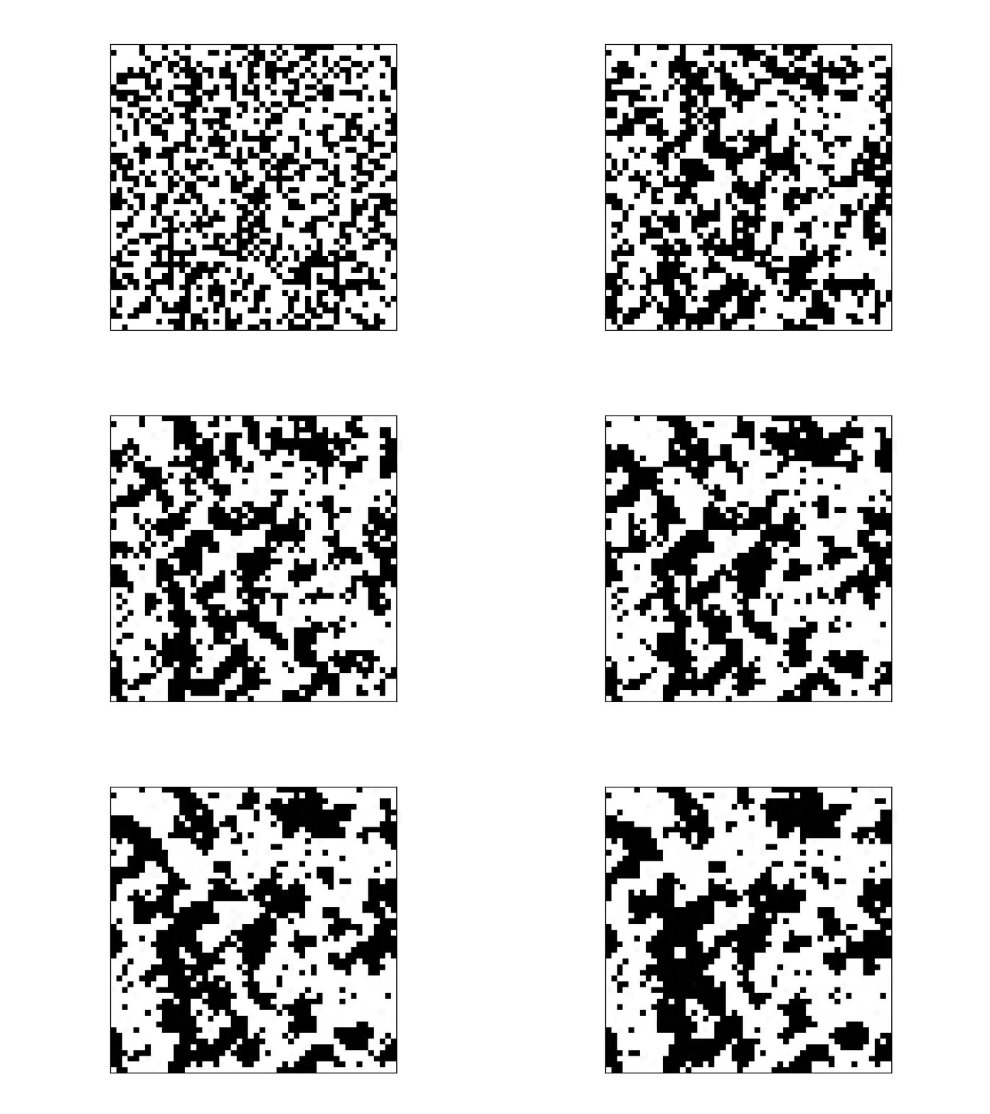
Modelling a Phase Change with Kawasaki Dynamics
Posted by christian on 15 September 2025
The Kawasaki dynamics formalism from statistical physics provides a simple model of a phase change (for example, the condensation of a gas at low enough temperature). Considering a gas of $N$ particles on a two-dimensional lattice of cells, a given configuration's energy can be calculated as the sum of the interaction energies between adjacent particles. The probability of this configuration (microstate) is $P \propto \exp\left(-E / T\right)$ (the Boltzmann formula where $T$ is the temperature.). At each step of the simulation select two cells at random. If exactly one contains a particle, then swapping them will lead to a change in microstate corresponding to a probability $P' \propto \exp\left(-E' / T\right)$ where $E'$ is the energy of the new configuration. The ratio of these probabilities is:
$$ q = \frac{P'}{P} = \exp\left(-\frac{E' - E}{T}\right) $$
but since at each step there is a choice of two configurations (by moving the particle to the empty cell or not) the sum of these probabilities must be unity, $P + P' = 1$. Therefore, $P = 1 / (1+q)$ and $P' = q/(1+q)$: that is, we should move the particle with a probability $q/(1+q)$. The code below implements this model simulation and shows a phase change occuring for low temperatures, whilst the particles remain in the gas phase for higher temperatures.

import numpy as np
import matplotlib.pyplot as plt
import matplotlib.animation as animation

ITERATIONS_PER_FRAME = 100
# Interaction energy.
Eint = 1
# Temperature.
T = 0.1
# Field size.
Nx, Ny = 50, 50
# Number of particles.
Np = 1000

arr = np.zeros(Nx * Ny)
# Choose Np random sites for the initial particle positions.
pjdx = np.random.choice(range(Nx * Ny), Np, replace=False)
arr[pjdx] = 1
arr = arr.reshape((Ny, Nx))

def get_arr_indexes(idx):
    ix = idx // Ny
    iy = idx - ix * Ny
    return ix, iy

def get_interaction_energy(ix, iy):
    """Return the interaction energy at field index (iy, ix)."""

    dirs = ((-1, -1), (0, -1), (1, -1),
            (-1, 0), (1, 0),
            (-1, 1), (0, 1), (1, 1))
    nneighbours = 0
    for (idx, idy) in dirs:
        if arr[(iy + idy) % Ny, (ix + idx) % Nx]:
            nneighbours += 1
    return -nneighbours * Eint

# The total interaction energy of the system...
#E = sum(get_interaction_energy(*get_arr_indexes(idx)) for idx in pjdx)
# ...relative to the starting energy
E = 0

def update_arr(arr, E):
    """
    Update the field by moving a particle into a vacant site,
    conditional that site's before and after interaction energy.
    """

    # Pick a particle by randomly choosing its index in pjdx.
    ipjdx1 = np.random.choice(range(Np))
    # pjdx1 is not the index into the flattened arr array giving
    # the particle's location in the field.
    pjdx1 = pjdx[ipjdx1]
    # Now pick a random vacant site.
    while True:
        # Pick a random site (which might be occupied).
        pjdx2 = np.random.choice(range(Nx * Ny), replace=False)
        if pjdx2 not in pjdx:
            # This site is vacant: we're done.
            break
    # Get the x,y indexes of the occupied and vacant sites.
    c1x, c1y = get_arr_indexes(pjdx1)
    c2x, c2y = get_arr_indexes(pjdx2)
    # Determine the interaction energy at the current occupied site.
    E1 = get_interaction_energy(c1x, c1y)
    # Determine the interaction energy if the vacant site were occupied.
    E2 = get_interaction_energy(c2x, c2y)

    q = np.exp(-(E2 - E1)/T)
    # With probability q / (1 + q), move the particle.
    if np.random.random() < q / (1 + q):
        pjdx[ipjdx1] = pjdx2
        arr[c2y, c2x] = 1
        arr[c1y, c1x] = 0
        E += E2 - E1
    return E

# Set up the plots.
fig, ax = plt.subplots()
im = ax.imshow(arr, cmap="binary")
ax.set_xticks([])
ax.set_yticks([])

def init():
    im.set_data(arr)
    return im,

def advance(i, E):
    for j in range(ITERATIONS_PER_FRAME):
        E = update_arr(arr, E)
    im.set_array(arr)
    return im,

nsec = 30
fps = 5
anim = animation.FuncAnimation(
                               fig,
                               advance,
                               fargs=(E,),
                               frames=nsec * fps,
                               interval=1000 / fps, # in ms
                               )
plt.show()