Measurements of the electron charge over time
Posted on 29 March 2021
In his 1986 book, Surely You're Joking, Mr. Feynman! physicist Richard Feynman writes:
We have learned a lot from experience about how to handle some of the ways we fool ourselves. One example: Millikan measured the charge on an electron by an experiment with falling oil drops, and got an answer which we now know not to be quite right. It's a little bit off because he had the incorrect value for the viscosity of air. It's interesting to look at the history of measurements of the charge of an electron, after Millikan. If you plot them as a function of time, you find that one is a little bit bigger than Millikan's, and the next one's a little bit bigger than that, and the next one's a little bit bigger than that, until finally they settle down to a number which is higher.
Why didn't they discover the new number was higher right away? It's a thing that scientists are ashamed of—this history—because it's apparent that people did things like this: When they got a number that was too high above Millikan's, they thought something must be wrong—and they would look for and find a reason why something might be wrong. When they got a number close to Millikan's value they didn't look so hard. And so they eliminated the numbers that were too far off, and did other things like that ...
He doesn't provide a citation for this, but the anecdote has become a standard example of confirmation bias and other psychological effects in scientific methodology.
This question on the StackExchange site History of Science and Mathematics has attracted some answers with scatter plots of the reported value of $e$ over time, but some of the citations are hard to track down or behind paywalls when they can be located.
The Python script below reads in the text file e-history.txt which summarizes the references I have been able to obtain, and plots the following graph in which the reported values and their uncertainties. These values are colour-coded according to the method used in the reporting article: in the first half of the 20th century the two main methods were oil-drop experiments like Millikan's (in)famous experiment or based on X-ray diffraction. By the 1940s the scientific consensus had settled close to the modern value, which (since the 2019 redefinition of the SI base units) has been fixed by definition as $1.602176634\times 10^{-19}\;\mathrm{C}$.
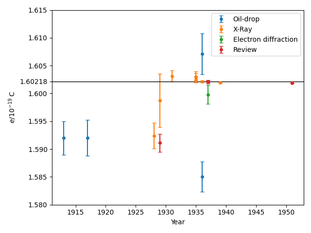 Image licensed under Creative Commons CC-BY-SA 4.0
The two data points from 1913 and 1917 are the original results found by Millikan, who has been accused of cherry-picking his data to reduce their reported uncertainty. Overall, the oil-drop experiments are the least accurate, mostly because of uncertainty in the value of the viscosity of air. Undoubtedly, the researchers reporting these experiments underestimated their errors.
Discounting the review article by antisemitic physical constant-botherer Raymond Birge, there are really only two non-oil-drop experiments that seem tied low to the Millikan value, and one of those has an error bar that overlaps the modern value. By the 1930s it was well accepted that the X-ray experiments provided a more accurate value for $e$.
| Year | Value /C | Reference |
|---|---|---|
| 1913 | 1.5920(30)×10-19 | R. A. Millikan, "On the Elementary Electrical Charge and the Avogadro Constant", Phys. Rev. 2, (1913): [doi] |
| 1917 | 1.5920(32)×10-19 | R. A. Millikan, "I. A New Determination of e, N, and Related Constants", The London, Edinburgh, and Dublin Philosophical Magazine and Journal of Science 34, (1917): [doi] |
| 1928 | 1.5924(23)×10-19 | A. P. R. Wadlund, "Absolute X-Ray Wave-Length Measurements", Phys. Rev. 32, (1928): [doi] |
| 1929 | 1.5911(16)×10-19 | R. T. Birge, "Probable Values of the General Physical Constants", Rev. Mod. Phys. 1, (1929): [doi] |
| 1929 | 1.5988(48)×10-19 | E. Bäcklin, "Eddington's Hypothesis and the Electronic Charge", Nature 123, (1929): [link] |
| 1931 | 1.6031(10)×10-19 | J. A. Bearden, "Absolute Wave-Lengths of the Copper and Chromium K-Series", Phys. Rev. 37, (1931): [doi] |
| 1935 | 1.60280(80)×10-19 | E. Bäcklin, "The X-Ray Crystal Scale, the Absolute Scale and the Electronic Charge", Nature 135, (1935): [link] |
| 1935 | 1.60230(17)×10-19 | J. A. Bearden, "The Measurement of X-Ray Wavelengths by Large Ruled Gratings", Phys. Rev. 48, (1935): [doi] |
| 1935 | 1.6030(10)×10-19 | M. Söderman, "Absolute value of the X-Unit", Nature 135, (1935): [link] |
| 1936 | 1.6071(37)×10-19 | G. Kellström, "Viscosity of Air and the Electronic Charge", Phys. Rev. 50, (1936): [doi] |
| 1936 | 1.5850(27)×10-19 | E. Bäcklin and H. Flemberg, "The Oil-Drop Method and the Electronic Charge", Nature 137, (1936): [link] |
| 1937 | 1.60210(17)×10-19 | R. T. Birge, "On the Values of Fundamental Atomic Constants", Phys. Rev. 52, (1937): [doi] |
| 1936 | 1.60210(17)×10-19 | R. T. Birge, "Interrelationships of e, h/e and e/m", Nature 137, (1936): [link] |
| 1937 | 1.5998(17)×10-19 | von Friesen, "", Uppsala Univ. Årsskr. 14, (1937): [doi] |
| 1937 | 1.60210(30)×10-19 | H. R. Robinson, "The charge of the electron", Rep. Prog. Phys. 4, (1937): [doi] |
| 1939 | 1.60194(13)×10-19 | F. G. Dunnington, "The Atomic Constants A Revaluation and an Analysis of the Discrepancy", Rev. Mod. Phys. 11, (1939): [doi] |
| 1951 | 1.601850(23)×10-19 | J. W. M. DuMond and E. R. Cohen, "Least-Squares Adjusted Values of the Atomic Constants as of December, 1950", Phys. Rev. 82, (1951): [doi] |
import re
import matplotlib.pyplot as plt

e = 1.602176634e-19

class Report:
    def __init__(self, citation, doi_or_url, data, method):
        self.citation = citation.strip()
        patt = '\((\d\d\d\d)\)'
        self.year = int(re.search(patt, citation).groups(1)[0])
        if doi_or_url == '-':
            self.doi_or_url = None
        else:
            self.doi_or_url = doi_or_url.strip()
        fields = data.split()
        self.value = float(fields[1])
        self.unc = float(fields[2])
        self.method = method.strip()

with open('e-history.txt') as fi:
    lines = fi.readlines()

reports = []
nreports = len(lines) // 5
for i in range(nreports):
    reports.append(Report(*lines[i*5:i*5+4]))
for report in reports:
    print(report.year, report.value, report.unc)

fig, ax = plt.subplots()
for method in ('Oil-drop', 'X-Ray', 'Electron diffraction', 'Review'):
    reps = [r for r in reports if r.method==method]
    ax.errorbar([report.year for report in reps],
                [report.value * 1.e19 for report in reps],
                yerr=[report.unc * 1.e19 for report in reps],
                marker='o', ls='', capsize=3, ms=4,
                label=method)
ax.axhline(e * 1.e19, c='k', lw=1)
ax.legend()
ax.set_ylim(1.58, 1.610)
ax.set_xlabel('Year')
ax.set_ylabel(r'$e / 10^{-19}\;\mathrm{C}$')
ax.set_yticks([1.58, 1.585, 1.59, 1.595, 1.6, e*1.e19, 1.605, 1.61, 1.615])
ax.set_yticklabels(['1.580', '1.585',' 1.590', '1.595', '1.600',
                    '1.60218', '1.605', '1.610', '1.615'])
plt.tight_layout()
plt.savefig('e-history.png')
plt.show()