Maze Generation by Cellular Automaton
Posted on 10 January 2018
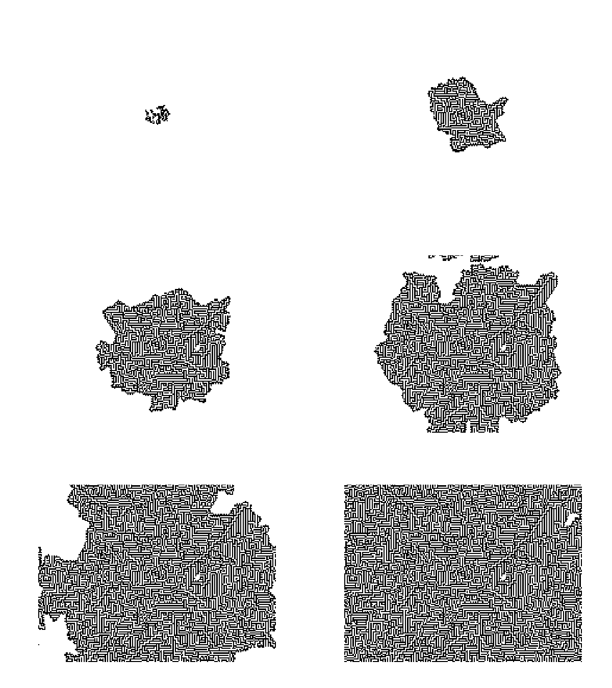
Cellular automata (CA) can be used to generate mazes, as described on the LifeWiki. A commonly used algorithm operates like John Conway's Game of Life in that a cell is born if it has exactly 3 neighbours but the survival rule is more liberal: a cell survives if it has 1–5 neighbours (rulestring B3/S12345).
The following code generates a maze using to this approach. The CA rules are implemented using SciPy's convolve2d algorithm to count neighbours. The code generates frame images of the growing maze every nit iterations, as animated below. The frames are saved to a subdirectory ca_frames.

This code is also available on my Github page.
# ca_maze.py
import numpy as np
from scipy.signal import convolve2d
import matplotlib.pyplot as plt

# Create a maze using the cellular automaton approach described at
# https://scipython.com/blog/maze-generation-by-cellular-automaton/
# The frames for animation of the growth of the maze are saved to
# the subdirectory ca_frames/.
# Christian Hill, January 2018.

def ca_step(X):
    """Evolve the maze by a single CA step."""

    K = np.ones((3, 3))
    n = convolve2d(X, K, mode='same', boundary='wrap') - X
    return (n == 3) | (X & ((n > 0) & (n < 6)))

# Maze size
nx, ny = 200, 150
X = np.zeros((ny, nx), dtype=np.bool)
# Size of initial random area (must be even numbers)
mx, my = 20, 16

# Initialize a patch with a random mx x my region
r = np.random.random((my, mx)) > 0.75
X[ny//2-my//2:ny//2+my//2, nx//2-mx//2:nx//2+mx//2] = r

# Total number of iterations
nit = 400
# Make an image every ipf iterations
ipf = 10

# Figure dimensions (pixels) and resolution (dpi)
width, height, dpi = 600, 450, 10
fig = plt.figure(figsize=(width/dpi, height/dpi), dpi=dpi)
ax = fig.add_subplot(111)

for i in range(nit):
    X = ca_step(X)
    if not i % ipf:
        print('{}/{}'.format(i,nit))
        im = ax.imshow(X, cmap=plt.cm.binary, interpolation='nearest')
        plt.axis('off')
        plt.savefig('ca_frames/_img{:04d}.png'.format(i), dpi=dpi)
        plt.cla()