Manufacturing Cobalt-60

Posted by: christian on 20 Nov 2021

(0 comments)

Lecture 12 of the MIT course 22.01: Introduction to Nuclear Engineering and Ionizing Radiation covers the manufacture of $\mathrm{^{60}Co}$ by neutron irradiation of $\mathrm{^{59}Co}$ in a research reactor. The thermal neutron absorption cross section of $\mathrm{^{59}Co}$ is $\sigma_0 \approx 20 \; \mathrm{barn}$, so for a neutron flux $\Phi$, the rate of change of the number of $\mathrm{^{59}Co}$ nuclei, $N_0$, may be written $$ \frac{\mathrm{d}N_0}{\mathrm{d}t} = -\sigma_0 \Phi N_0 \quad\Rightarrow N_0(t) = N_0(0)\mathrm{e}^{-\sigma_0\Phi t} $$

The $\mathrm{^{60}Co}$ nuclei produced in this process undergo natural beta-decay with a half-life $t_{1/2} = 1925.4\;\mathrm{days}$ to the stable isotope, $\mathrm{^{60}Ni}$, and, potentially, neutron absorption with a cross section $\sigma_1$. Denoting the number of $\mathrm{^{60}Ni}$ as $N_1$:

$$ \frac{\mathrm{d}N_1}{\mathrm{d}t} = \sigma_0 \Phi N_0 - \sigma_1 \Phi N_1 - \lambda_1 N_1, $$ where $\lambda_1 = \ln 2 / t_{1/2}$. This differential equation can be solved with the introduction of the integrating factor $\exp[(\sigma_1\Phi + \lambda_1)t]$ since:

\begin{align*} & \exp[(\sigma_1\Phi + \lambda_1)t]\frac{\mathrm{d}N_1}{\mathrm{d}t} + (\sigma_1 \Phi + \lambda_1) N_1\exp[(\sigma_1\Phi + \lambda_1)t] = \sigma_0 \Phi N_0\exp[(\sigma_1\Phi + \lambda_1)t]\\ \Rightarrow \quad& \frac{\mathrm{d}}{\mathrm{d}t}\left[ \exp[(\sigma_1\Phi + \lambda_1)t] N_1 \right] = \sigma_0 \Phi N_0(0)\exp[(\sigma_1\Phi - \sigma_0\Phi + \lambda_1)t] \\ \Rightarrow \quad & \exp[(\sigma_1\Phi + \lambda_1)t] N_1(t) = \frac{\sigma_0 \Phi N_0(0)}{\sigma_1\Phi - \sigma_0\Phi + \lambda_1}\left[ \exp[(\sigma_1\Phi - \sigma_0\Phi + \lambda_1)t] - 1 \right]\\ \Rightarrow \quad & N_1(t) = \frac{\sigma_0 \Phi N_0(0)}{\sigma_1\Phi - \sigma_0\Phi + \lambda_1}\left[\exp(- \sigma_0\Phi t) - \exp[-(\sigma_1\Phi + \lambda_1)t] \right]. \end{align*}

(There appears to be a sign error in the videoed lecture for this derivation).

In principle, the $\mathrm{^{60}Ni}$ could capture a neutron as well, but the cross section for this process is rather small.

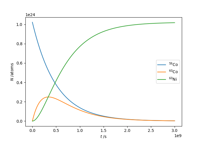
This Jupyter Notebook calculates and plots the amounts of these isotopes as a function of time in a reactor with isotropic neutron flux, $\Phi = 10^{14}\;\mathrm{n\,cm^{-2}\,s^{-1}}$, and determines the maximum amount of $\mathrm{^{60}Co}$ created from an initial amount of 100 g of $\mathrm{^{59}Co}$. $\sigma_1$ is small and taken to be 0.

import numpy as np
from scipy.optimize import minimize
import matplotlib.pyplot as plt
from scipy.constants import N_A

# Neutron absorption cross section for 59Co, cm2.
sigma0 = 20 * 1.e-24
# Neutron absorption cross section for 60Co.
sigma1 = 0

# Half-life (days) and decay constant for 60Co, s-1.
thalf1 = 1925.4
lam1 = np.log(2) / (thalf1 * 24 * 60 * 60)

# Neutron flux, cm2.s-1.
Phi = 1.e14
# Mass of 59Co sample, g.
m59Co = 100
# Atomic mass of 59Co, Da.
M59Co = 58.9
# Number of 59Co atoms
N00 = m59Co / M59Co * N_A

def N0(t):
    """Amount of 59Co as a function of time."""
    return N00 * np.exp(-sigma0 * Phi * t)

def N1(t):
    """Amount of 60Co as a function of time."""
    d = Phi * (sigma1 - sigma0) + lam1
    return sigma0 * Phi * N00 / d * (np.exp(-sigma0*Phi*t) - np.exp(-(sigma1*Phi + lam1)*t))

def N2(t):
    """Amount of 60Ni as a function of time."""
    return N00 - N0(t) - N1(t)

def dN1dt(t):
    """Rate of change of 60Co as a function of time."""
    return sigma0 * Phi * N0(t) - N1(t) * (sigma1 * Phi + lam1)

# Plot the isotope amounts up to tmax seconds.
tmax = 3.e9
t = np.linspace(0, tmax, 1000)
plt.plot(t, N0(t), label='$\mathrm{^{59}Co}$')
plt.plot(t, N1(t), label='$\mathrm{^{60}Co}$')
plt.plot(t, N2(t), label='$\mathrm{^{60}Ni}$')
plt.xlabel('$t$ /s')
plt.ylabel('$N$ /atoms')

The problem set associated with the course also suggests finding the optimum amount of time to irradiate the $\mathrm{^{59}Co}$ to maximise the profit from the $\mathrm{^{60}Co}$ generated, assuming a reactor time cost of USD 1000 per day and a $\mathrm{^{60}Co}$ price of USD 100 per $\mathrm{\mu Ci}$.

# Cost of reactor, USD.s-1.
CR = 1.e3 / 24 / 60 / 60
# Price of 60Co, Bq-1.
CI = 100 * 1.e6 / 3.7e10

def I(t):
    """The predicted net income from the 60Co after time t in the reactor (USD)."""
    # Calculate the activity of 60Co as A1 = lam1.N1.
    return -CR * t + CI * lam1 * N1(t)

def dIdt(t):
    """dI/dt in USD/sec."""
    return -CR + CI * lam1 * dN1dt(t)

The maximum profit can be found as the minimum of $-I$.

from scipy.optimize import minimize
minimize(lambda t: -I(t), 0.5e9, jac = lambda t:-dIdt(t))

      fun: -2806888567702.389
 hess_inv: array([[42765.86838808]])
      jac: array([-7.46765967e-06])
  message: 'Optimization terminated successfully.'
     nfev: 21
      nit: 6
     njev: 21
   status: 0
  success: True
        x: array([3.38753637e+08])

This turns out to be the same time as would produce the maximum amount of $\mathrm{^{60}Co}$ possible, presumably because USD 1000 per day is an unrealistically cheap cost for the reactor time during production and omits other considerations (such as isotopic separation and opportunity costs).

topt = 3.388e8 / 60 / 60 / 24 / 365
print(f'{topt:.1f} yrs')

10.7 yrs

• ← Changing the palette of an image
• The Klein–Nishina formula →