Linear transformations on the two-dimensional plane
Posted on 09 September 2019
A linear transformation in two dimensions can be visualized through its effect on the two orthonormal basis vectors $\hat{\imath}$ and $\hat{\jmath}$. In general, it can be represented by a $2 \times 2$ matrix, $\boldsymbol{T}$, which acts on a vector $v$ to map it from a vector space spanned by one basis onto a different vector space spanned by another basis: $\boldsymbol{v'} = \boldsymbol{T}\boldsymbol{v}$. This change of basis can be visualized by drawing the basis vectors in the two-dimensional plane, along with equally-spaced "grid lines" parallel to each of them. A linear transformation keeps the grid lines evenly spaced, and the origin fixed.
The following code produces a visualization of the effect of a linear transformation by plotting the grid lines, basis vectors and the unit square (or whatever parallelogram it ends up as) before and after the transformation.
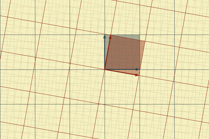
Example 1: Rotation by $\theta = 10^\circ$: $$ T = \left( \begin{array}{rr} \cos\theta & -\sin\theta\\ \sin\theta & \cos\theta \end{array} \right) $$
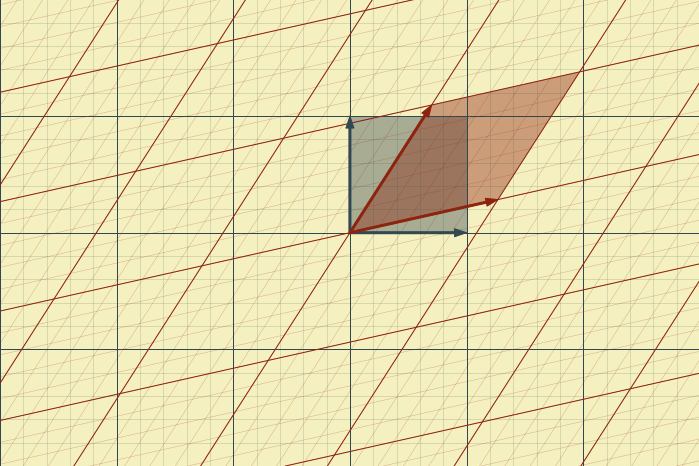
Example 2: Rotation by 10° followed by a shear:
$$
T = \left(
\begin{array}{rr}
\frac{6}{5} & \frac{1}{2}\\[1ex]
\frac{1}{2} & \frac{6}{5}
\end{array}
\right)
\left(
\begin{array}{rr}
\cos\theta & -\sin\theta\\
\sin\theta & \cos\theta
\end{array}
\right)
$$
The code allows the appearance of the plot to be altered by customizing the constants defined at the start.
import numpy as np
import matplotlib.pyplot as plt

# Figure settings: background, reference grid, translated grid.
BACKGROUND_COLOUR = '#fff5c8'
BACKGROUND_COLOUR = '#f5f0c0'
REF_COLOUR = '#324851'
TRANS_COLOUR = '#8d230f'
# Reference grid limits (-XMAX, XMAX), (-YMAX, YMAX); number of minor grids
# per unit reference grid interval.
XMAX, YMAX = np.array((3, 2))
NMINOR = 5

# Styles for the major and minor grid lines.
major_styles = {'lw': 1}
minor_styles = {'lw': 0.5, 'alpha': 0.3}

# Set up the plot, turning off the axis labels and ensuring squares are square.
DPI = 72
WIDTH_PIXELS = 700
width_inches = WIDTH_PIXELS / DPI
height_inches = width_inches * YMAX / XMAX

# The reference orthonormal basis vectors, i and j.
ivec, jvec = np.array((1,0)), np.array((0,1))

def get_intersection(p, r, q, s):
    """Determine the intersection point of two lines, if any.

    The lines are defined by the vector equations p + αr and q + βs, where
    r and s are parallel to the lines. α may take any (real) value; but
    0 ≤ β ≤ 1: we are only interested in the intersection of the first line
    with a segment of the second, representing a boundary line of the plot
    rectangle.
    Returns either the position of the intersection, or None if there is none.

    """

    def _cross(v, w):
        """A two-dimensional "cross product" of vectors v and w."""
        return v[0]*w[1] - v[1]*w[0]

    rxs = _cross(r, s)
    if rxs == 0:
        # The lines are parallel.
        return None
    u = _cross(q-p, r) / rxs
    if 0 <= u <= 1:
        # Intersection with the line segment
        return q + u*s
    # Fall through and return None if the intersection is outside the segment.

def get_intersections(p, r):
    """Get all the intersections of the line p + αr with the boundary."""

    # The vectors q and s for the boundary line segments, q +  βs for 0 ≤ β ≤ 1
    xvec, yvec = XMAX * ivec, YMAX * jvec
    boundary_lines = [np.array((xvec - yvec, 2*yvec)),
                      np.array((xvec + yvec, -2*xvec)),
                      np.array((-xvec + yvec, -2*yvec)),
                      np.array((-xvec - yvec, 2*xvec))]

    # Find all the interesections: we expect either none or 2.
    intersections = []
    for q, s in boundary_lines:
        t = get_intersection(p, r, q, s)
        if t is not None:
            intersections.append(t)
    return intersections

def plot_grid(ax, ivec, jvec, fac, c=REF_COLOUR, **kwargs):
    """Plot a the grid defined by the basis vectors ivec and jvec.

    fac determines how many grid lines to draw per multiple of ivec and jvec.
    c is the line colour; other arguments are handed on to ax.plot.

    """

    def plot_grid_lines(v, w, c=REF_COLOUR, **kwargs):
        """Plot the grid lines corresponding to kv + w and -kv + w.

        Keep incrementing k until a grid line no longer intersects the plot
        boundary. c is the line colour; other arguments get passed to ax.plot.

        """
        k = 0
        while True:
            intersections = get_intersections(k * v, w)
            if len(intersections) < 2:
                return
            ax.plot(*np.array(intersections).T, c, **kwargs)
            # Plot this grid line's "mirror image" for k -> -k, unless k=0.
            if k:
                intersections = get_intersections(-k * v, w)
                ax.plot(*np.array(intersections).T, c, **kwargs)
            k += 1

    # Plot the grid lines parallel to ivec and jvec.
    plot_grid_lines(jvec / fac, ivec, c, **kwargs)
    plot_grid_lines(ivec / fac, jvec, c, **kwargs)

def show_vector(ax, tip, tail=(0,0), c='k'):
    """Display a vector from tail to tip as an arrow with colour c."""
    arrowprops={'color': c, 'headwidth': 8, 'width': 2}
    ax.annotate(s='', xy=tip, xytext=tail, arrowprops=arrowprops)

def show_unit_square(ax, ivec, jvec, c='k'):
    """Display the unit "square" (parallelogram) defined by ivec, jvec."""

    kwargs = {'edgecolor': 'none', 'facecolor': c, 'alpha': 0.4}
    path = [(0,0), ivec, ivec+jvec, jvec]
    sq = plt.Polygon(path, **kwargs)
    ax.add_patch(sq)

def transform_basis(T, ivec, jvec):
    """Return a transformed basis by applying the matrix transformation T."""
    return T @ np.vstack((ivec, jvec))

def rotate_basis(theta, ivec, jvec):
    """A special case of a linear transformation: rotation by theta radians."""
    c, s = np.cos(theta), np.sin(theta)
    R = np.array(((c, -s),(s, c)))
    return transform_basis(R, ivec, jvec)

def plot_grids(ivec, jvec, ivecp, jvecp, draw_basis=True,
               draw_unit_square=True, filename='grids.png'):

    fig, ax = plt.subplots(figsize=(width_inches, height_inches))
    fig.patch.set_facecolor(BACKGROUND_COLOUR)
    ax.set_facecolor(BACKGROUND_COLOUR)
    ax.axis('off')
    ax.set_aspect('equal')

    # Plot the reference grid.
    plot_grid(ax, ivec, jvec, NMINOR, **minor_styles)
    plot_grid(ax, ivec, jvec, 1, **major_styles)

    # Plot the transformed basis grid.
    plot_grid(ax, ivecp, jvecp, NMINOR, c=TRANS_COLOUR, **minor_styles)
    plot_grid(ax, ivecp, jvecp, 1, c=TRANS_COLOUR, **major_styles)

    # Show the basis vectors and unit square for the reference grid.
    if draw_basis:
        show_vector(ax, ivec, c=REF_COLOUR)
        show_vector(ax, jvec, c=REF_COLOUR)
    if draw_unit_square:
        show_unit_square(ax, ivec, jvec, c=REF_COLOUR)

    # Show the basis vectors and their parallelogram for the transformed grid.
    if draw_basis:
        show_vector(ax, ivecp, c=TRANS_COLOUR)
        show_vector(ax, jvecp, c=TRANS_COLOUR)
    if draw_unit_square:
        show_unit_square(ax, ivecp, jvecp, c=TRANS_COLOUR)

    # Set the Axes limits, and remove all padding from the figure.
    ax.set_xlim(-XMAX, XMAX)
    ax.set_ylim(-YMAX, YMAX)
    plt.subplots_adjust(left=0, right=1, top=1, bottom=0)

    plt.savefig(filename, dpi=DPI, facecolor=BACKGROUND_COLOUR)
    plt.show()

# Rotate the basis vectors and then transform by an addition matrix, T.
ivecp, jvecp = rotate_basis(np.radians(10), ivec, jvec)
plot_grids(ivec, jvec, ivecp, jvecp, filename='grids2.png')

T = np.array(((1.2, 0.5),(0.5, 1.2)))
ivecp, jvecp = transform_basis(T, ivecp, jvecp)
plot_grids(ivec, jvec, ivecp, jvecp, filename='grids1.png')