Least-squares fitting to an exponential function
Posted on 13 January 2022
Many phenomena can be described in terms of a measured variable varying exponentially with a quantity. For example, a processes such as radioactive decay and first-order reaction rates are described by an ordinary differential equation of the form
$$ \frac{\mathrm{d}y}{\mathrm{d}t} = -ky $$
where $t$ is time, $y(t)$ is, e.g. the number of radioactive nuclei or reactant molecules present at time $t$ and $k$ is a constant describing the rate of the decay or reaction.
This simple equation leads to an exponential dependence of $y(t)$:
$$ y(t) = y(0)e^{-kt}, $$
where $y(0)$ is the initial condition of the system (e.g. number of radioactive nuclei) at $t=0$.
When presented with (possibly noisy) data of $y$ at a series of discrete time points, the common way of determining the parameters $y(0)$ and $k$ is to linearize the problem by taking logs:
$$ \ln y(t) = \ln y(0) -kt. $$
One can therefore plot the natural logarithm of the measured values of $y$ as a function of $t$ and obtain the best fit straight line through these points: the gradient and intercept of this line give $-k$ and $\ln y(0)$, respectively.
The nonlinear problem has become a linear one of the form:
$$ y = a + bx, $$
and the problem of obtaining the optimum (best fit) parameters $a$ and $b$ from $n$ data points $(x_k, y_k)$ ($k=1,2,\ldots, n$) is open to ordinary linear least squares fitting (i.e. algebraically, rather than from a line of best-fit judged by eye). The approach is to minimize the squared residual error,
$$ r^2 = \sum_{k=1}^n (y_k -a -bx_k)^2. $$
Solving the pair of equations $\partial r^2 / \partial a = 0$ and $\partial r^2 / \partial b = 0$ gives the result:
$$ a = \frac{S_{xx}S_y - S_{xy}S_x}{nS_{xx} - S_x^2} \; \mathrm{and} \; b = \frac{nS_{xy} - S_xS_y}{nS_{xx} - S_x^2}, $$ where $$ S_x = \sum_{k=1}^n x_k, \quad S_y = \sum_{k=1}^n y_k, \quad S_{xx} = \sum_{k=1}^n x_k^2, \quad\mathrm{and}\;S_{xy} = \sum_{k=1}^n x_k y_k. $$
This process gives the best fit (in a least squares sense) to the model function, $y = a + bx$, provided the uncertainties (errors) associated with the measurements, $y_k$ are drawn from the same gaussian distribution, with the same width parameter, $\sigma$.
However, when the exponential function is linearized as above, not all of the errors associated with the measurements, $y_k$, are treated equally (since $\ln (y_k + \delta_k) \neq \ln y_k + \ln \delta_k$): taking the logarithm of the data points biases the least squares fit implemented using the method above, since greater weight is distributed to smaller values of $y_k$. That is, the parameters retrieved that best fit $\ln y = \ln a + bx$ are not those that best fit the function $y = ae^{bx}$.
In practice, in most situations, the difference is quite small (usually smaller than the uncertainty in either set of the fitted parameters), but the correct optimum parameters to the exponential fit can be obtained either by using a weighted least squares fit (where the weights are taken to be $y_k$ in the common case that $\sigma_k = \sqrt{y_k}$), or (in the case of a constant $\sigma$) by taking the approximate values of $a$ and $b$ from a regular least-squares fit and using them as the initial guesses to a nonlinear fit of $y = ae^{bx}$.
The equations determining the true optimum parameters, $a$ and $b$, in the case of a constant uncertainty parameter for all values of $y_k$, are derived from the requirement to minimise the function
$$ r^2 = \sum_{k=1}^n ( y_k - ae^{bx} )^2 $$
with respect to $a$ and $b$. This two-dimensional problem can be reduced to a one dimensional minimization as follows: first solve $\partial r^2 / \partial a = 0$ for $a$:
$$ \frac{\partial r^2}{\partial a} = -2\sum_{k=1}^n e^{bx_k}( y_k - ae^{bx_k}) = 0 \quad \Rightarrow \; a = \frac{\sum_{k=1}^n e^{bx_k}y_k}{\sum_{k=1}^n e^{2bx_k}} = \frac{S_1}{S_2}. $$
Then write the condition for minimization of $r^2$ with respect to $b$, treating $a$ as a function of $b$:
$$ \frac{\partial r^2}{\partial b} = -2\sum_{k=1}^n ( y_k - ae^{bx_k} ) \left[ \frac{\mathrm{d}a}{\mathrm{d}b}e^{bx_k} + a x_k e^{bx_k} \right] = 0. $$
The problem is then one of finding the solution to
$$ \sum_{k=1}^n ( y_k - ae^{bx_k} ) \left[ \frac{\mathrm{d}a}{\mathrm{d}b} + a x_k \right]e^{bx_k} = 0, $$
where
$$ \frac{\mathrm{d}a}{\mathrm{d}b} =\frac{1}{S_2^2}\left[ S_2 \frac{\mathrm{d}S_1}{\mathrm{d}b} - S_1\frac{\mathrm{d}S_2}{\mathrm{d}b} \right]; \quad \frac{\mathrm{d}S_1}{\mathrm{d}b} = \sum_{k=1}^n x_k y_k e^{bx_k}, \quad \frac{\mathrm{d}S_2}{\mathrm{d}b} = 2\sum_{k=1}^n x_k e^{bx_k}. $$
A general-purpose root-finding algorithm such as Newton-Raphson is usually suitable.
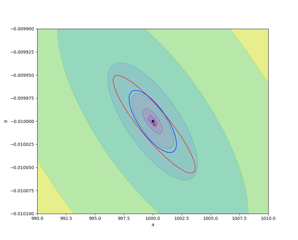
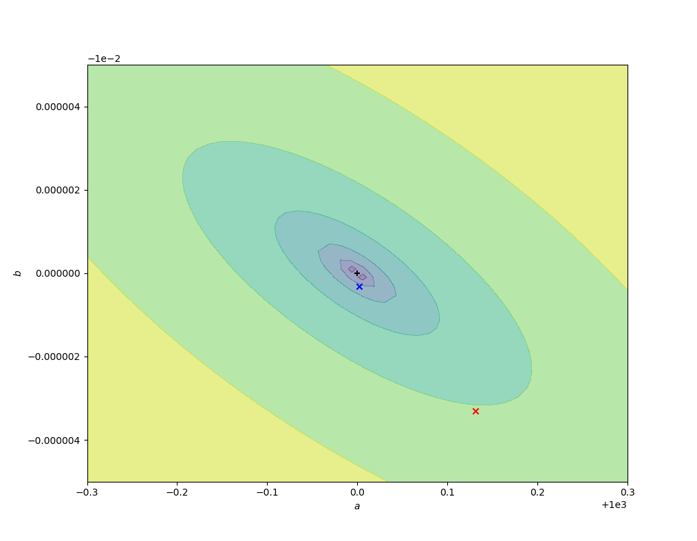
The code below compares the naive ordinary least squares fit on some sample log-transformed data with the above nonlinear fit. In the figures below, the contours are of values of $r^2(a, b)$, decreasing to a minimum at the exact values chosen for the simulation (black cross). The red cross and curve are the average best fit value (over 10000 fits) and confidence ellipse (one standard deviation) for the linear fit, and the blue cross and curve are the same for the nonlinear fit. Better results are obtained from the nonlinear fit, as expected, but (for this data set) the difference is small compared to the parameter uncertainties.
import numpy as np
from scipy.optimize import newton, minimize, least_squares
import matplotlib.pyplot as plt
from matplotlib.patches import Ellipse
import matplotlib.transforms as transforms
from confidence_ellipse import confidence_ellipse

np.random.seed(2)

def log_transformed_fit(x, y):
    """Ordinary linear least-squares fit to ln(y) = ln(a) + bx."""

    lny = np.log(y)

    Sx = np.sum(x)
    Sy = np.sum(lny)
    Sxx = np.sum(x**2)
    Sxy = np.sum(x * lny)

    den = n * Sxx - Sx**2
    a = (Sy * Sxx - Sxy * Sx) / den
    b = (n*Sxy - Sy*Sx) / den

    return (np.exp(a), b)


def direct_nonlinear_fit(x, y, prms0):
    """Direct nonlinear two-dimensional least-squares fit to y = a.exp(bx)."""

    def func(prms, x, y):
        a, b = prms
        return (a * np.exp(b * x) - y)**2

    res = least_squares(func, prms0, args=(x, y))
    return res.x


def nonlinear_one_dimension_fit(x, y, prms0):
    """Indirect nonlinear fit to y = a.exp(bx), treating a = a(b)."""

    def r2(b, x, y):
        S1 = np.sum(y * np.exp(b * x))
        S2 = np.sum(np.exp(2 * b * x))
        a = S1 / S2
        return np.sum( (y - a * np.exp(b * x))**2 )


    def get_a_and_dadb(b, x, y):
        S1 = np.sum(y * np.exp(b * x))
        S2 = np.sum(np.exp(2 * b * x))
        dS1db = np.sum(x * y * np.exp(b * x))
        dS2db = np.sum(2 * x * np.exp(2 * b * x))
        a = S1 / S2
        dadb = (S2 * dS1db - S1 * dS2db) / S2**2
        return a, dadb

    def dr2db(b, x, y):
        a, dadb = get_a_and_dadb(b, x, y)
        fac1 = y - a * np.exp(b * x)
        fac2 = dadb + a * x
        return -2 * np.sum(fac1 * np.exp(b * x) * fac2)

    b0 = prms0[1]
    # Use Newton-Raphson to find the root of dr2/db.
    b = newton(dr2db, b0, args=(x, y))
    a, _ = get_a_and_dadb(b, x, y)
    return a, b


y0, k = 1000, -0.01

# Repeat the fit M times using each method
M = 10000
a1, b1 = np.empty((2, M))
a2, b2 = np.empty((2, M))

# The (constant) width of the Gaussian noise to add.
sigma = y0 * 0.005
# The exact function, on a grid of n data points.
n = 50
x = np.linspace(0, 200, n)
yexact = y0 * np.exp(k * x)
for i in range(M):
    # Generate some data to fit by adding random noise.
    y = yexact + np.random.standard_normal(n) * sigma
    # Do the fit it two ways.
    a, b = log_transformed_fit(x, y)
    a1[i], b1[i] = a, b
    a, b = nonlinear_one_dimension_fit(x, y, (a, b))
    #a, b = direct_nonlinear_fit(x, y, (a, b))
    a2[i], b2[i] = a, b

# Calculate the mean values of the fitted parameters, a and b, by each method.
a1mean, b1mean = a1.mean(), b1.mean()
a2mean, b2mean = a2.mean(), b2.mean()

print(f'Exact parameter values, (a, b)   : {(y0, k)}')
print(f'log-transformed linear fit values: {(a1mean, b1mean)}')
print(f'nonlinear fit values             : {(a2mean, b2mean)}')

fig, ax = plt.subplots()

# Contour plot of the cost function, r2(a, b).
da = 0.01
amin, amax = y0 * (1 - da), y0 * (1 + da)
db = 0.01
bmin, bmax = k * (1 - db), k * (1 + db)
a, b = np.linspace(amin, amax, 50), np.linspace(bmin, bmax, 50)
A, B = np.meshgrid(a, b)
y = y0 * np.exp(k * x)
r2 = np.sum((y - A[:, :, None] * np.exp(B[:, :, None] * x))**2, axis=2)
r2 = np.log(r2)

ax.contourf(A, B, r2, alpha=0.5)

ax.scatter(a1mean, b1mean, c='r', marker='x')

# 1-sigma confidence ellipses for the fitted data.
confidence_ellipse(a1, b1, ax, 1, edgecolor='r')
confidence_ellipse(a2, b2, ax, 1, edgecolor='b')

ax.scatter(a2mean, b2mean, c='b', marker='x')
ax.scatter(y0, k, c='k', marker='+')

ax.set_xlabel(r'$a$')
ax.set_ylabel(r'$b$')

plt.show()
This code requires the following function, confidence_ellipse, from the Matplotlib gallery of examples.
def confidence_ellipse(x, y, ax, n_std=3.0, facecolor='none', **kwargs):
    """
    Create a plot of the covariance confidence ellipse of *x* and *y*.

    Parameters
    ----------
    x, y : array-like, shape (n, )
        Input data.

    ax : matplotlib.axes.Axes
        The axes object to draw the ellipse into.

    n_std : float
        The number of standard deviations to determine the ellipse's radiuses.

    **kwargs
        Forwarded to `~matplotlib.patches.Ellipse`

    Returns
    -------
    matplotlib.patches.Ellipse
    """
    if x.size != y.size:
        raise ValueError("x and y must be the same size")

    cov = np.cov(x, y)
    pearson = cov[0, 1]/np.sqrt(cov[0, 0] * cov[1, 1])
    # Using a special case to obtain the eigenvalues of this
    # two-dimensionl dataset.
    ell_radius_x = np.sqrt(1 + pearson)
    ell_radius_y = np.sqrt(1 - pearson)
    ellipse = Ellipse((0, 0), width=ell_radius_x * 2, height=ell_radius_y * 2,
                      facecolor=facecolor, **kwargs)

    # Calculating the stdandard deviation of x from
    # the squareroot of the variance and multiplying
    # with the given number of standard deviations.
    scale_x = np.sqrt(cov[0, 0]) * n_std
    mean_x = np.mean(x)

    # calculating the stdandard deviation of y ...
    scale_y = np.sqrt(cov[1, 1]) * n_std
    mean_y = np.mean(y)

    transf = transforms.Affine2D() \
        .rotate_deg(45) \
        .scale(scale_x, scale_y) \
        .translate(mean_x, mean_y)

    ellipse.set_transform(transf + ax.transData)
    return ax.add_patch(ellipse)