Langton's ant on a hexagonal plane
Posted on 22 November 2020
Langton's ant is a two-dimensional cellular automaton usually implemented on a square grid in which each cell has one of two states (white or black). The ant moves according to the simple rules:
(1) on a white square turn 90° clockwise flip the square to black, and advance one square;
(2) on a black square turn 90° anticlockwise, flip the square to white, and advance one square.
This formulation is easily coded and some interesting, complex emergent behaviour results; if the simulation is allowed to proceed for long enough, it apparently always converges on the same unbounded, repeating "highway" pattern, whatever the original configuration of the grid:
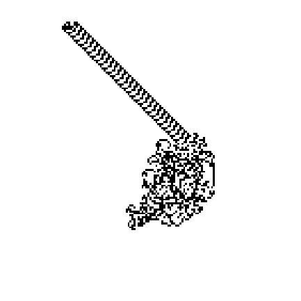
The code producing this image is as follows:
import numpy as np
import matplotlib.pyplot as plt

def square_ant(nx, ny, nmoves, filename='langton.png'):
    """Langton's ant simulation for nmoves on a (nx, ny) square grid."""

    # The ant's universe: a (nx, ny) grid of squares, initially all black (0).
    arr = np.zeros((ny, nx), dtype=np.uint8)

    # Figure resolution and dimensions.
    DPI = 100
    width, height = 500, 500
    fig = plt.figure(figsize=(width/DPI, height/DPI), dpi=DPI, facecolor='k')
    ax = fig.add_subplot()
    ax.set_facecolor('k')
    # Ensure squares are square, remove padding from around Axes.
    plt.axis('equal')
    plt.subplots_adjust(top=1, bottom=0, right=1, left=0, hspace=0, wspace=0)

    # The ant starts at the centre of the grid, facing "east".
    ix, iy = nx // 2, ny // 2
    dx, dy = 1, 0
    for i in range(nmoves):
        if arr[iy,ix]:
            # White square: turn clockwise.
            dx, dy = dy, -dx
        else:
            # Black square: turn anticlockwise.
            dx, dy = -dy, dx
        # Flip the square colour, advance one square.
        arr[iy,ix] = 1 - arr[iy,ix]
        ix, iy = ix+dx, iy+dy

    # Depict the final state of the grid as a black-and-white image.
    ax.imshow(arr, cmap='Greys', interpolation='nearest')
    plt.savefig('langton.png', dpi=DPI)
    plt.show()

# The size of the grid and number of moves the ant is to take.
nx, ny = 175, 175
nmoves = 13000
square_ant(nx, ny, nmoves)
There are various ways to generalize the above rules; the popular one described here involves replacing the square grid with a hexagonal one, and the two white/black states replaced with a larger number, each corresponding to a chosen "move" to an adjacent cell.
Following the notation of the linked Wikipedia article, the moves are labeled as follows:
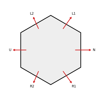
An $n$-state automaton can then be described by a sequence of $n$ such moves.
The easiest way to represent the hexagonal grid in a NumPy array is to treat it as square grid with every other row displaced. Although it means indexing into the array differently for odd- and even-numbered rows in order to get the displacements to the adjacent cells, no additional memory is required.
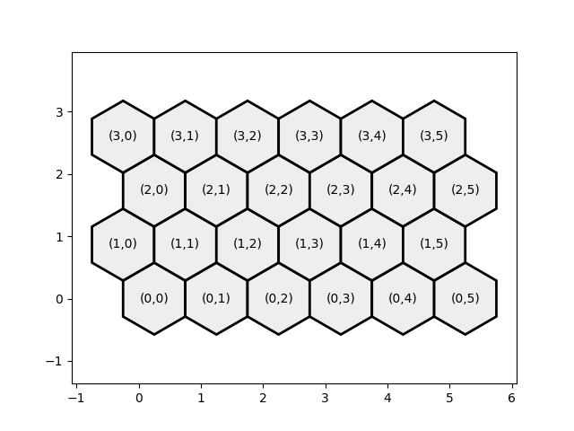
For example, the change in row and column indices involved in the move "L2" from a cell (say, (2, 3)) in an even-numbered row is (+1, 0); for the same move from a cell (say, (1, 3)) in an odd-numbered rows it is (+1, -1). More information about implementing hexagonal grids is available on this excellent website.
Some pleasing images can be produced by colouring the cells according to their state after the ant has been wandering around for a few thousand steps. This is the pattern produced by the rule L2NNL1L2L1 over 83,000 steps:
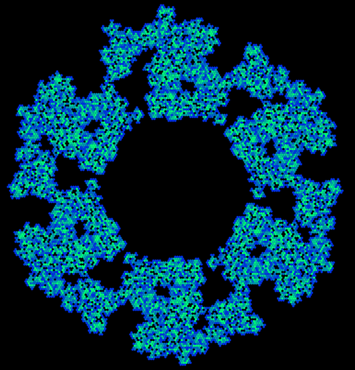
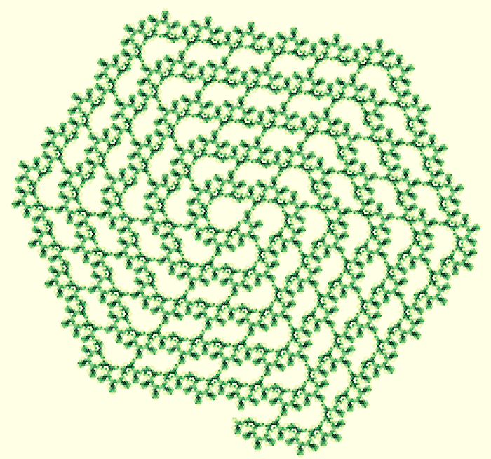
The rule R1R2NUR2R1L2 generates a pleasing, fractal-like spiral:
The code and some examples are given here:
import numpy as np
import matplotlib.pyplot as plt

def hex_ant(n1, n2, nmoves, rules_string, initial_position=None, cmap='hot',
            filename=None):
    """Langton's ant simulation for nmoves on a (n1, n2) hex grid.

    The movement rules are given as a string of the basic commands:
    N, L2, L1, U, R2, R1 corresponding to the moves made in each of
    the states the hexagonal cells can be in. The cells are coloured
    according to their state using the provided colormap, cmap.

    initial_position is a tuple (i1, i2) of the ant's starting position; if not
    provided, the and starts off in the middle of the grid.

    If not provided, the image filename will be <rules_string>.png.

    """

    def plot_hex(ax, i1, i2, c='#888888'):
        """Draw the hexagon indexed at (i2, i1) in colour c on Axes ax."""

        # Scaling factor: separate the centre of the hexagons by this amount.
        s = 1
        # Hexagon side-length.
        a = s / np.sqrt(3)
        # Hexagon centre (cx, cy), and vertex coordinates.
        cx, cy = s*i1 + s/4 * (-1)**(i2%2), 3*a/2*i2
        x1, y1 = cx, cy + a
        x2, y2 = cx + s/2, cy + a/2
        x3, y3 = cx + s/2, cy - a/2
        x4, y4 = cx, cy - a
        x5, y5 = cx - s/2, cy - a/2
        x6, y6 = cx - s/2, cy + a/2
        hexagon = plt.Polygon(((x1, y1), (x2, y2), (x3, y3), (x4, y4),
                               (x5, y5), (x6, y6)), fc=c)
        ax.add_patch(hexagon)

    arr = np.zeros((n2, n1), dtype=np.uint8)

    # Moves for even and odd rows, clockwise, starting with <- ("west").
    moves = np.array([ [(-1,0), (0,1), (1,1), (1,0), (1,-1), (0,-1)],
                       [(-1,0), (-1,1), (0,1), (1,0), (0,-1), (-1,-1)]
                     ])

    def parse_rules_string(s):
        """Parse the string of rules.

        The rule string sequence provided is parsed into a sequence of indexes
        into the array moves, e.g. the rule 'L2' resolves to -2: to move
        anticlockwise by 120 deg, change the movement to the one two places
        earlier (mod 6) in the moves array; the rule 'N' resolves to 0: to
        keep heading in the same direction, don't change the movement rule.

        """

        move_dict = {'N': 0, 'L2': -2, 'L1': -1, 'R1': 1, 'R2': 2, 'U': 3}
        rules = []
        i = 0
        while i < len(s):
            t = s[i]
            if t in 'LR':
                i += 1
                t += s[i]
            try:
                rules.append(move_dict[t])
            except KeyError:
                raise ValueError('Unidentified move {} in rules {}'
                                 .format(t, s))
            i += 1
        return rules

    # Figure resolution and dimensions.
    DPI = 100
    width, height = 1000, 1000
    fig = plt.figure(figsize=(width/DPI, height/DPI), dpi=DPI, facecolor='k')
    ax = fig.add_subplot()
    # Ensure squares are square, remove padding from around Axes.
    plt.axis('equal')
    plt.subplots_adjust(top=1, bottom=0, right=1, left=0, hspace=0, wspace=0)

    rules = parse_rules_string(rules_string)
    # Retrieve the colours to use for each cell state from the chosen colormap.
    nrules = len(rules)
    cm = plt.get_cmap(cmap)
    c = [cm(i/(nrules-1)) for i in range(nrules)]
    # We're not going to plot hexagons for the cells with state 0: just colour
    # the background this colour instead.
    ax.set_facecolor(c[0])

    i1, i2 = initial_position or (n1 // 2, n2 // 2)
    # j indexes the moves array for a given row parity: as the ant turns
    # we update j, which determines d1, d2, the change in coordinates (i1, i2)
    # of the ant.
    j = 0
    for i in range(nmoves):
        j = (j + rules[arr[i2,i1]]) % 6
        d1, d2 = moves[i2%2, j]
        arr[i2,i1] = (arr[i2,i1] + 1) % nrules
        i1, i2 = i1 + d1, i2 + d2
        if i1 < 0 or i1 >= n1 or i2 < 0 or i2 >= n2:
            # if the ant leaves the grid, bail on the simulation.
            print('Ant left the grid.')
            break

    # Plot the final state of the grid.
    for i1 in range(n1):
        for i2 in range(n2):
            if arr[i2,i1] > 0:
                # Only plot a hexagon if its state is not zero.
                plot_hex(ax, i1, i2, c[arr[i2,i1]])

    ax.set_xlim(0, n1)
    ax.set_ylim(0, n2)

    if not filename:
        filename = rules_string + '.png'
    plt.savefig(filename, dpi=DPI)
    plt.show()

rules_string = 'R1R2NUR2R1L2'   # spiral
n1, n2 = 250, 250
nmoves = 64000
hex_ant(n1, n2, nmoves, rules_string, cmap='YlGn')

#rules_string = 'L2NNL1L2L1'     # ring
#n1, n2 = 250, 250
#initial_position = n1 // 3, 7 * n2 // 8
#nmoves = 83000
#hex_ant(n1, n2, nmoves, rules_string, initial_position, cmap='hot',
#        filename='ring.png')


# Slowly-expanding maze.
#rules_string = 'L1L1R1'
#n1, n2 = 150, 150
#nmoves = 10000
#hex_ant(n1, n2, nmoves, rules_string, cmap='autumn')

# Blob.
#rules_string = 'L2NUL2R1R2NL1L2'
#n1, n2 = 150, 150
#nmoves = 100000
#initial_position = n1 // 3, 5 * n2 // 6
#hex_ant(n1, n2, nmoves, rules_string, cmap='plasma')
An online implementation of various generalizations of Langton's ant is here.