Iceberg dynamics
Posted on 22 February 2021
Prompted by this tweet and campaign for icebergs to be depicted in their most stable equilibrium orientation, here is a Python script modelling the dynamics of a two-dimensional iceberg which starts in an arbitrary orientation and position and relaxes under gravitational and buoyant forces to its most stable configuration. A cork floats "on its side": with its longest axis parallel to the water's surface (it doesn't bob around with its longest axis vertical), and an iceberg does the same.
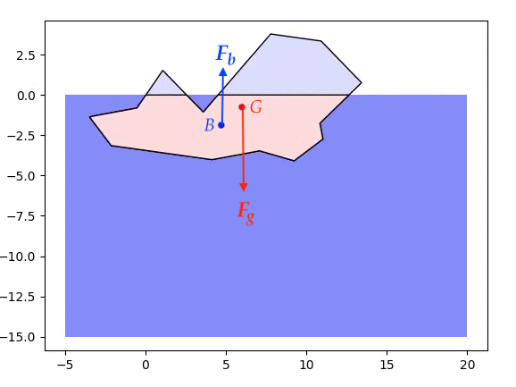
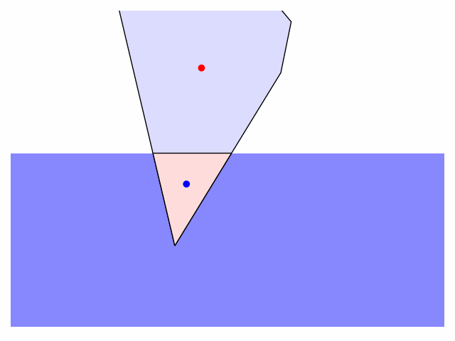
The centre of mass ($G$) and the centre of buoyancy ($B$, the centre of mass of the displaced water) are indicated by the red and blue dots respectively. The motion of the iceberg (treated as a rigid body) is dictated by the force of gravity ($\boldsymbol{F}_g$) and an opposing buoyant force ($\boldsymbol{F}_b$) due to the displaced water. In addition to any translational force moving the centre of mass of the iceberg, where these forces are not colinear they exert a torque, $\boldsymbol{\tau} = \boldsymbol{r} \times \boldsymbol{F}_b$, where $r$ is the vector from $G$ to $B$, which tends to rotate the iceberg.
There are few things one can customize in the code: the shape of the iceberg (defined as a sequence of vertex coordinates), the initial position ($h$) and orientation (call rotate_poly to rotate the iceberg to a given angle), and the friction applied to damp the rotation and translation of the iceberg in water (edit the apply_friction function). I'll tidy up and post the code on GitHub when I get a moment.
import numpy as np
import matplotlib.pyplot as plt
from matplotlib import animation

# Plot limits: ideally the figure will not have to rescale during the animation
xmin, xmax = -5, 20
ymin, ymax = -10, 8
width, height = xmax - xmin, ymax - ymin

# The area density of sea water and ice.
rho_water, rho_ice = 1.027, 0.9
# Acceleration due to gravity, m.s-2
g = 9.81

def canonicalize_poly(xy):
    """Shift the (N+1,2) array of coordinates xy to start at minimum y."""
    #if get_area(xy) > 0:
    #    xy = xy[::-1]
    idx_ymin = xy[:,1].argmin()
    xy = np.roll(xy[:-1], -idx_ymin, axis=0)
    return np.vstack((xy, xy[0]))

def rotate_poly(xy, theta):
    """Rotate the (N+1,2) array of coordinates xy by angle theta about (0,0).

    The rotation angle, theta, is in radians.

    """
    s, c = np.sin(theta), np.cos(theta)
    R = np.array(((c, -s), (s, c)))
    xyp = (R @ xy.T).T
    return canonicalize_poly(xyp)

def get_area(xy):
    """Return the area of the polygon xy.

    xy is a (N+1,0) NumPy array defining the N polygon vertices, but repeating
    the first vertex as its last element. The "shoelace algorithm" is used.

    """

    x, y = xy.T
    return np.sum(x[:-1]*y[1:] - x[1:]*y[:-1]) / 2

def get_cofm(xy, A=None):
    """Return the centre of mass of the polygon xy.

    xy is a (N+1,0) NumPy array defining the N polygon vertices, but repeating
    the first vertex as its last element. If the polygon area is not passed
    in as A it is calculated. The polygon must have uniform density.

    """

    if A is None:
        A = get_area(xy)
    x, y = xy.T
    Cx = np.sum((x[:-1] + x[1:]) * (x[:-1]*y[1:] - x[1:]*y[:-1])) / 6 / A
    Cy = np.sum((y[:-1] + y[1:]) * (x[:-1]*y[1:] - x[1:]*y[:-1])) / 6 / A
    return np.array((Cx, Cy))

def get_moi(xy, rho):
    """Return the moment of inertia of the polygon xy with density rho.

    xy is a (N+1,0) NumPy array defining the N polygon vertices, but repeating
    the first vertex as its last element.

    """

    x, y = xy.T
    Ix = rho * np.abs(np.sum((x[:-1]*y[1:] - x[1:]*y[:-1]) *
                (y[:-1]**2 + y[:-1]*y[1:] + y[1:]**2)) / 12)
    Iy = rho * np.abs(np.sum((x[:-1]*y[1:] - x[1:]*y[:-1]) *
                (x[:-1]**2 + x[:-1]*x[1:] + x[1:]**2)) / 12)
    # Perpendicular axis theorem.
    Iz = Ix + Iy
    return Ix, Iy, Iz

def get_zero_crossing(pts):
    """Return the coordinates of the zero-crossing in pts.

    pts is a pair of (x, y) points, assumed to be joined by a straight line
    segment. This function returns the coordinates (x,0) at which this line
    crosses the y-axis (corresponding to sea-level in our model).

    """
    P0, P1 = pts
    x0, y0 = P0
    x1, y1 = P1
    if (x1-x0) == 0:
        return x1, 0
    m = (y1-y0)/(x1-x0)
    c = y1 - m*x1
    return -c/m, 0

def get_displaced_water_poly(iceberg, submerged=None):
    """Get the polygon for the submerged portion of the iceberg.

    iceberg is a (N+1,2) array of coordinates corresponding to the iceberg's
    vertexes in its current position and orientation (the first vertex is
    repeated at the end of the array);
    submerged is a boolean array corresponding to the vertexes which are
    under water (<0); if not provided it is calculated.

    """

    if submerged is None:
        submerged = (iceberg[:,1] <= 0)
    nsubmerged = sum(submerged)

    # Partially-submerged iceberg: find where it enters the sea, i.e. which
    # edges cross zero. zc_idx holds the indexes of the vertices *before*
    # each zero-crossing edge.
    diff = np.diff(submerged)
    zc_idx = np.where(diff)[0]
    # Interpolate to find the coordinates of the zero crossing.
    ncrossings = len(zc_idx)
    # We're going to build a polygon for the shape of the displaced water,
    # i.e. the submerged part of the iceberg.
    displaced_water = np.empty((nsubmerged + ncrossings, 2))
    # Loop over the points *before* each crossing in pairs. NB if the
    # iceberg is partially submerged, len(zc_idx) is guaranteed to be even.
    assert not ncrossings % 2
    i = j  = 0
    for idx1, idx2 in zip(zc_idx[0::2], zc_idx[1::2]):
        # All the submerged vertices up to the upwards crossing.
        displaced_water[j:j+idx1-i+1] = iceberg[i:idx1+1]
        # Work out where the crossing vertex should be and add it.
        c = get_zero_crossing(iceberg[idx1:idx1+2])
        j += idx1 - i + 1
        displaced_water[j] = c
        j += 1

        # Now the downward crossing: all the unsubmerged vertices are
        # skipped, and an extra vertex at sea level is added.
        c = get_zero_crossing(iceberg[idx2:idx2+2])
        displaced_water[j] = c
        j += 1
        i = idx2 + 1
    # Copy across any remaining submerged vertexes to displaced_water.
    displaced_water[j:] = iceberg[i:]
    return displaced_water

def apply_friction(omega, dh):
    """Apply frictional forces to the angular and linear velocities."""

    # Hard friction: angular and linear velocities are immediately quenched.
    # after movement.
    # return 0, np.array((0,0))

    # Intermediate friction: reduce the velocities by some fraction.
    return omega * 0.95, dh * 0.65


# Our two-dimensional iceberg, defined as a polygon.
poly = [(0,0), (5, -4), (5, -7), (1, -18), (-5, -5)]

# Repeat the initial vertex at the end, for convenience.
iceberg0 = np.array(poly + [poly[0]])
# Centre the iceberg's local coordinates on its centre of mass.
iceberg0 = iceberg0 - get_cofm(iceberg0)
# We might want to start the iceberg off in some different orientation:
# if so, rotate it here.
iceberg0 = rotate_poly(iceberg0, -0.2)

# Get the (signed) area, mass, and weight of the iceberg.
A = get_area(iceberg0)
M = rho_ice * abs(A)
Fg = np.array((0, -M * g))

# We also need the Iz component of the iceberg's moment of inertia.
_, _, Iz = get_moi(iceberg0, rho_ice)

fig, ax = plt.subplots()
ax.set_xlim(xmin, xmax)
ax.set_ylim(ymin, ymax)
# We would prefer equal distances in the x- and y-directions to look the same.
ax.axis('equal')
ax.axis('off')
fig.tight_layout()

# The centre of mass starts at this height above sea level.
h = 5
# theta is the turning angle of the iceberg from its initial orientation;
# G is the position of its centre of mass (in world coordinates).
theta, G = 0, np.array((6, h))
# omega = dtheta / dt is the angular velocity; dh is the linear velocity.
omega, dh = 0, np.array((0,0))
# The time step (s): small, but not too small.
dt = 0.1

def update(it):
    """Update the animation for iteration number it."""

    global omega, dh, G, theta

    print('iteration #{}'.format(it))

    # Update iceberg orientation and position.
    theta += omega * dt
    G = G + dh * dt

    # Rotate and translate a copy of the original iceberg into its current.
    # position.
    iceberg = rotate_poly(iceberg0, theta)
    iceberg = iceberg + G

    # Which vertices are submerged (have their y-coordinate negative)?
    submerged = (iceberg[:,1] <= 0)
    nsubmerged = sum(submerged)

    iceberg_in_water = True
    if nsubmerged in (0, 1):
        # The iceberg is in the air above the surface of the sea.
        B = None
        Adisplaced = 0
        alpha = 0
        iceberg_in_water = False

    if iceberg_in_water:
        # Apply some frictional forces which damp the motion in water.
        omega, dh = apply_friction(omega, dh)
        if nsubmerged == len(submerged):
            # The iceberg is fully submerged.
            displaced_water = iceberg
            Adisplaced = A
            B = G
        else:
            displaced_water = get_displaced_water_poly(iceberg, submerged)

            # Area of the displaced water and position of the centre of buoyancy.
            Adisplaced = get_area(displaced_water)
            B = get_cofm(displaced_water)

    # Buoyant force due to the displaced water.
    Fb = np.array((0, rho_water * abs(Adisplaced) * g))

    if B is not None:
        # Vector from G to B
        r = B - G
        # Torque about G
        tau = np.cross(r, Fb)
        alpha = tau / Iz

    # Resultant force on the iceberg.
    F = Fg + Fb
    # Net linear acceleration.
    a = F / M

    # Now plot the scene for this frame of the animation.
    ax.clear()

    # The sea! The sea!
    sea_patch = plt.Rectangle((xmin, ymin), width, -ymin, fc='#8888ff')
    ax.add_patch(sea_patch)

    # The iceberg itself, in its current orientation and position.
    poly_patch = plt.Polygon(iceberg, fc='#ddddff', ec='k')
    ax.add_patch(poly_patch)

    if B is not None:
        # Draw the submerged part of the iceberg in a different colour.
        poly_patch = plt.Polygon(displaced_water, fc='#ffdddd', ec='k')
        ax.add_patch(poly_patch)

        # Indicate the position of the centre of buoyancy.
        bofm_patch = plt.Circle(B, 0.2, fc='b')
        ax.add_patch(bofm_patch)

    # Indicate the position of the centre of mass.
    cofm_patch = plt.Circle(G, 0.2, fc='r')
    ax.add_patch(cofm_patch)

    # Update the angular and linear velocities
    omega += alpha * dt
    dh = dh + a * dt

    ax.set_xlim(xmin, xmax)
    ax.set_ylim(ymin, ymax)
    ax.axis('off')

ani = animation.FuncAnimation(fig, update, 300, blit=False, interval=100, repeat=True)
plt.show()