A quick project inspired by this tweet by @story645 referencing Jacques Bertin's Semiology of Graphics.

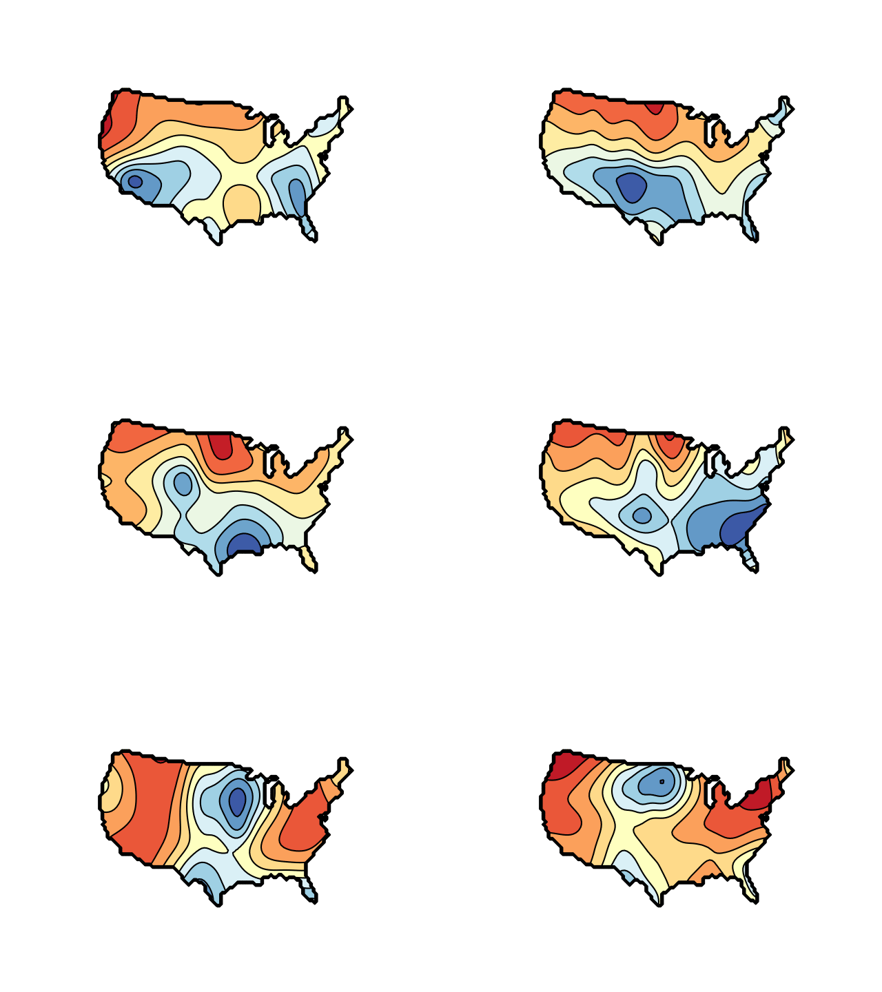
The function plotted is the sum of a random selection of two-dimensional Gaussian functions, with filled and line contours indicated using Matplotlib's contourf and contour methods. They are animated by changing the Gaussians' parameters in random steps.

The plot is constrained to the region defined by a mask array, read in as a PNG image file. Examples files are us_100.png and france_100.png. Mask images are assumed to be have RGB and alpha channels.

import numpy as np
import matplotlib.pyplot as plt
import matplotlib.animation as animation
from PIL import Image

SAVE_ANIMATION = False

# The mask image to use: only plot contours on the black area.
img = Image.open('us_100.png')
mask = np.array(img)[::-1,:,:].mean(axis=2) < 128

# Number of 2D Gaussian functions to use, size of the plot array.
ng = 80
nx, ny = 100, 100
arr = np.zeros((nx, ny))

# Scaling factors for random initialization of Gaussian parameters.
sigma = 20
A = 1
g_prms = np.array(
                 (np.random.random(ng) * nx,
                  np.random.random(ng) * ny,
                  sigma * (np.random.random(ng) + 0.2),
                  sigma * (np.random.random(ng) + 0.2),
                  A * np.random.random(ng))
                 )

# Meshgrid of 2D coordinates.
x, y = np.arange(0, nx), np.arange(0, ny)
X, Y = np.meshgrid(x, y)

def gaussian(prms):
    """Return the 2D Gaussian function defined by prms."""
    x0, y0, sig_x, sig_y, A = prms
    return A[:,None,None] * np.exp(
                - ((X-x0[:,None,None]) / sig_x[:,None,None])**2
                - ((Y-y0[:,None,None]) / sig_y[:,None,None])**2
                                  )
# Initialize the array with the initial Gaussian parameters.
arr = np.sum(gaussian(g_prms), axis=0)

# Start the figure, make sure it's square and turn off the Axes labels.
fig, ax = plt.subplots()
ax.axis('equal')
ax.axis('off')

# Plot the filled and line contours, and the outline of the mask.
cf = ax.contourf(arr, cmap='RdYlBu')
c = ax.contour(arr, colors='k')
ax.contour(mask, colors='k')

# These parameters determine how fast the Gaussian parameters change.
vx, vy = 4, 4
vsig_x, vsig_y = 0.2, 0.2
vA = 0.05
sc = np.array((vx, vy, vsig_x, vsig_y, vA)).reshape(5, 1)

def animate(i):
    """Set the data for the ith iteration of the animation."""

    global c, cf, arr, g_prms

    # Advance the parameters, update the array, and apply the mask.
    g_prms += sc * (1 - 2*np.random.random((5, ng)))
    arr = np.sum(gaussian(g_prms), axis=0)
    arr[~mask] = np.nan
    # Update the plot objects: remove the previous collections to save memory.
    for coll in cf.collections:
        coll.remove()
    cf = ax.contourf(arr, cmap='RdYlBu')
    for coll in c.collections:
        coll.remove()
    c = ax.contour(arr, colors='k')
    return c, cf

if SAVE_ANIMATION:
    anim = animation.FuncAnimation(fig, animate, frames=100, repeat=False)
    anim.save('us.gif', writer='imagemagick', fps=5)
else:
    anim = animation.FuncAnimation(fig, animate, frames=100)
    plt.show()