A quartic oscillator
Posted on 10 May 2018
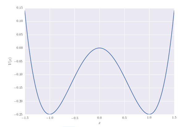
A oscillator whose potential energy is given as a function of the displacement, $x$, as $V(x) = \frac{1}{4}kx^4 - \frac{1}{2}kx^2$ may be modelled by finding the numerical solution to the ordinary differential equation $$ F = m\ddot x = - \frac{\mathrm{d}V}{\mathrm{d}x}. $$ In the following, for simplicity we assumethat $m=1\; \mathrm{kg}$ and $k=1\;\mathrm{N\,m^{-1}}$ (alternatively, we could apply a coordinate transformation to arbitrary values of $m$ and $k$, and measure time, position and energy in some suitable transformed units). The potential, $V(x)$ has two symmetric wells at $x=\pm 1$ of depth $V=-\frac{1}{4}$ separated by a barrier at $x=0$ where $V(0)=0$. The behviour of the oscillator is equivalent to the motion of a particle on this potential energy surface.
First, some imports:
import numpy as np
from scipy.integrate import odeint, quad
from scipy.optimize import brentq
import matplotlib.pyplot as plt
from matplotlib import animation, rc
import seaborn as sbs
rc('font', **{'family': 'serif', 'serif': ['Computer Modern'], 'size': 20})
rc('text', usetex=True)
rc('animation', html='html5')
Define the potential, and its first derivative (which we need later) as callables:
V = lambda x: 0.5 * x**2 * (0.5 * x**2 - 1)
dVdx = lambda x: x**3 - x
And plot it:
# The potential energy function on a grid of x-points.
xgrid = np.linspace(-1.5, 1.5, 100)
Vgrid = V(xgrid)
plt.plot(xgrid, Vgrid)
plt.xlabel('$x$')
plt.ylabel('$V(x)$')
The numerical solution uses scipy.integrate.odeint:
def deriv(X, t):
    """Return the derivatives dx/dt and d2x/dt2."""

    x, xdot = X
    xdotdot = -dVdx(x)
    return xdot, xdotdot

def solve(tmax, dt, x0, v0):
    """Solve the equation of motion for a quartic oscillator.

    Find the numerical solution to the quartic oscillator equation
    of state using a suitable time grid: tmax is the maximum time
    to integrate to; dt is the sampling interval.
    x0, v0 are the initial position and velocity.

    Returns the time grid, t, and position, x, and velocity,
    xdot, packed into the n x 2 array X.

    """

    # The time grid
    t = np.arange(0, tmax, dt)
    # Initial conditions: x, xdot
    X0 = [x0, v0]
    X = odeint(deriv, X0, t)
    return t, X
The initial condition is taken to be specified by an initial position, $x_0$, with zero velocity ($v_0 \equiv \dot x_0 = 0$). Since the potential is symmetric about $x=0$, we will consider $x_0 > 0$ only. If the particle starts with $E = V(x_0) < 0$ then it never leaves the righthand well; for E > 0 it oscillates symmetrically about the origin, exploring both wells.
We would like to know the period of the motion, which we can obtain by numerical integration. The time it takes the particle to move from $x=a$ to $x=b$ is: $$ \Delta t = \int_{t_a}^{t_b} \mathrm{d}t = \int_{a}^{b} \frac{\mathrm{d}t}{\mathrm{d}x}\,\mathrm{d}x = \frac{1}{\sqrt{2}}\int_{a}^{b} \frac{\mathrm{d}x}{\sqrt{E- V(x)}}, $$ where we have used $v = \mathrm{d}x/\mathrm{d}t = \sqrt{\frac{2}{m}(E-V(x))}$, since $E = \frac{1}{2}mv^2 + V(x)$.
For $E>0$ the period is $$ T = \frac{4}{\sqrt{2}}\int_0^{x_0} \frac{\mathrm{d}x}{\sqrt{E- V(x)}}. $$ If $E<0$, we need to find the second turning point within the well, $x_1$, (which we can do numerically) and the period is $$ T = \frac{2}{\sqrt{2}}\int_{x_0}^{x_1} \frac{\mathrm{d}x}{\sqrt{E- V(x)}}. $$ Here is the code (change the value of $x_0$ for different initial conditions). We will integrate for three periods of the motion.
# Set up the motion for a oscillator with initial position
# x0 and initially at rest. The potential is symmetric about
# x=0, so it's reasonable to insist that the user sets x0 > 0.
x0, v0 = 1.42, 0

# Total energy. If this is negative, the system never
# gets over the central barrier
E = V(x0)
print('E = {:.2f}'.format(E))

# This is the function we need to integrate to find the period.
def f(x):
    return 1/np.sqrt(E - V(x))

if E > 0:
    # The particle makes it over the barrier.
    A = x0
    # Get the period of the motion by numerical integration.
    T = 4 / np.sqrt(2) * quad(f, 0, A)[0]
else:
    # The particle oscillates inside the righthand well:
    # find the other turning point and integrate to get the
    # period.
    if x0 < 1:
        x1 = brentq(lambda x: E-V(x), 1, 1.5)
    else:
        # Don't forget to make sure x0 < x1.
        x0, x1 = brentq(lambda x: E-V(x), 0, 1), x0
    T = np.sqrt(2) * quad(f, x0, x1)[0]

print('Period, T = {:.2f} s'.format(T))

# Maximum time to integrate to, time step.
tmax, dt = 3*T, T/1000
Now solve the differential equation and check the numerical value of the period matches our calculation:
t, X = solve(tmax, dt, x0, v0)
x, xdot = X.T
dx, dxdot = x-x0, xdot-v0
pstep = np.argmin(np.hypot(dx, dxdot)[1:]) + 1
print('Period, T = {:.2f} s'.format(t[pstep]))
In the Jupyter Notebook provided on my github page, various properties of the particle are presented as an animation: the particle's potential energy and its position as a function of time, as well as its position in phase space $(x, \dot x)$ as a function of time. A Poincaré section is also plotted: the particle's motion is periodic, so the path it takes in phase space is closed and the Poincaré section, plotted as $(x, \dot x)$ for each period of the motion, is a single point.
# The animation
fig, ax = plt.subplots(nrows=2,ncols=2)
ax1 = ax[0,0]
ax1.plot(xgrid, Vgrid)
ln1, = ax1.plot([], [], 'mo')
ax1.set_xlabel(r'$x / \mathrm{m}$')
ax1.set_ylabel(r'$V(x) / \mathrm{J}$')

# Position as a function of time
ax2 = ax[1,0]
ax2.plot(t,x)
ax2.set_xlabel(r'$t / \mathrm{s}$')
ax2.set_ylabel(r'$x / \mathrm{m}$')
ln2, = ax2.plot([], [], 'mo')

# Phase space plot
ax3 = ax[1,1]
ax3.plot(x, xdot)
ax3.set_xlabel(r'$x / \mathrm{m}$')
ax3.set_ylabel(r'$\dot{x} / \mathrm{m\,s^{-1}}$')
ln3, = ax3.plot([], [], 'mo')

# Poincaré section plot
ax4 = ax[0,1]
ax4.set_xlabel(r'$x / \mathrm{m}$')
ax4.set_ylabel(r'$\dot{x} / \mathrm{m\,s^{-1}}$')
scat1 = ax4.scatter([x0], [v0], s=45, lw=0, c='m')
# We need to set the x- and y-limits otherwise the animation
# doesn't work.
ax4.set_xlim(ax3.get_xlim())
ax4.set_ylim(ax3.get_ylim())
plt.tight_layout()

def animate(i):
    """Update the image for iteration i of the Matplotlib animation."""

    ln1.set_data(x[i], V(x[i]))
    ln2.set_data(t[i], x[i])
    ln3.set_data(x[i], xdot[i])
    if not i % pstep:
        scat1.set_offsets(X[:i+1:pstep])
    return

anim = animation.FuncAnimation(fig, animate, frames=len(x), interval=1)