Fitting a Gaussian Function

The Doppler broadening of spectral lines is caused by the distribution of their velocities relative to the absorbed or emitted photon and, in the absence of other broadening mechanisms (pressure broadening, lifetime broadening, instrument resolution effects, etc.) results in a Gaussian line profile:

$$ f_\mathrm{G}(\nu; \nu_0, \alpha_\mathrm{D}) = \sqrt{\frac{\ln 2}{\alpha_\mathrm{D}^2\pi}} \exp\left[ -\ln 2\frac{(\nu - \nu_0)^2}{\alpha_\mathrm{D}^2}\right], $$

where $\nu_0$ is the transition frequency (central frequency of the line), and the half-width at half-maximum,

$$ \alpha_\mathrm{D} = \sqrt{\frac{2k_\mathrm{B}T\ln 2}{mc^2}}\nu_0 $$

for an absorbing species of mass $m$ and temperature, $T$.

The high-resolution spectrum of a low-density gas can therefore be used as a thermometer if isolated spectral lines can be fit to a Gaussian function. Conversely, before its value was fixed by definition, such a fit to a spectrum taken at a known temperature was one way of measuring the Boltzmann constant, $k_\mathrm{B}$.

The file NH3-line.csv contains the high-resolution spectrum of the $\nu_2\;\mathrm{saQ}(6,3)$ rovibrational line of the principal isotopologue of ammonia ($\mathrm{{}^{14}N^{1}H_3}$), which is well-separated from other absorptions. We can analyse this spectrum to determine the temperature of the gas.

import numpy as np
from scipy.optimize import curve_fit
import matplotlib.pyplot as plt

def fG(nu, nu0, alphaD):
    """Normalized Gaussian function with HWHM alphaD, centered on nu0."""
    N = np.sqrt(np.log(2) / np.pi) / alphaD
    return N * np.exp(-np.log(2) * ((nu - nu0) / alphaD)**2)

# Read in the data file
nu, spec = np.genfromtxt('NH3-line.csv', delimiter=',', unpack=True, skip_header=1)

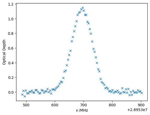
At this stage, it makes sense to plot the experimental data to see if we can make an educated guess for the values of the parameters we want to fit:

plt.plot(nu, spec, 'x')
plt.xlabel(r'$\nu\;/\mathrm{MHz}$')
plt.ylabel(r'Optical Depth')

$The experimental spectrum of the $\nu_2\;\mathrm{saQ}(6,3)$ rovibrational line of ammonia$

The function to fit is actually $f(\nu) = A f_\mathrm{G}(\nu)$, since the optical depth depends on the product of the path length, absorber density, line strength and the lineshape function. We will absorb the other factors into the parameter $A$:

def f(nu, A, nu0, alphaD):
    return A * fG(nu, nu0, alphaD)

There is some noise, but we can get good estimates of the parameter values from inspecting the spectrum:

A_guess = 1.2
nu0_guess = nu[np.argmax(spec)]
alphaD_guess = 40
popt, pcov = curve_fit(f, nu, spec, p0=(A_guess, nu0_guess, alphaD_guess))
A, nu0, alphaD = popt
A, nu0, alphaD

(100.33655618951202, 28953694.49912839, 41.66608989340652)

The $1\sigma$ standard deviations in these parameters are given by the square root of the diagonal elements of the covariance matrix:

pstd = np.sqrt(np.diag(pcov))
sigma_A, sigma_nu0, sigma_alphaD = pstd
sigma_A, sigma_nu0, sigma_alphaD

(0.5656240531671611, 0.23034846010693605, 0.27120953083941735)

The fitted parameters are therefore:

\begin{align*} A &= 100.34(57)\\ \nu_0 &= 28953694.50(23) \;\mathrm{MHz}\\ \alpha_\mathrm{D} &= 41.67(27) \;\mathrm{MHz} \end{align*}

The temperature can now be retrieved from the defintion of $\alpha_\mathrm{D}$.

from scipy.constants import c, k as kB, u

# Isotope masses, mass of (14N)(1H)3, in kg.
mH, mN = 1.007825031898 * u, 14.003074004 * u
m = mN + 3*mH

b = m * c**2 / 2 / kB / np.log(2)
T = b * (alphaD / nu0)**2
T

274.93872647125903

If we ignore correlations between the fitted parameters, the uncertainty in the retrieved temperature can be calculated by propagating the fit uncertainties:

sigma_T = 2 * T * np.sqrt(
    (sigma_alphaD / alphaD)**2 + (sigma_nu0 / nu0)**2)
sigma_T

3.5792176902931563

We might report the temperature as $T = 274.9 \pm 3.6\;\mathrm{K}$ therefore.

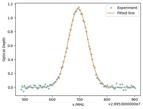
The fitted line profile can be plot along with the data as follows:

plt.plot(nu, spec, '+', label='Experiment')
plt.plot(nu, f(nu, *popt), label='Fitted line')
plt.xlabel(r'$\nu\;/\mathrm{MHz}$')
plt.ylabel(r'Optical Depth')
plt.legend()
plt.plot()

Observed and fitted Gaussian line shape for an ammonia rovibrational transition

E34.3: Fitting a Gaussian Function