30: Fitting the Vibrational Spectrum of CO

Analysing a rovibrational spectrum

The high-resolution infrared absorption spectrum of a typical diatomic molecule will show signals due to rovibrational transitions between its energy levels. Real molecules are anharmonic oscillators, and bands corresponding to a change in vibrational quantum number, \(\Delta v = 0, 1, 2,\ldots\) can be observed, given sufficient sensitivity, though the fundamental band \(v=0 \rightarrow v=1\) is expected to be by far the strongest. Each band consists of individual transition lines involving a change in rotational quantum number, \(\Delta J = \pm 1\) (for a closed-shell diatomic molecule). The collection of lines with \(\Delta J = -1\) are referred to as the P-branch; those with \(\Delta J = +1\) form the R-branch.

The files, CO-v01.txt and CO-v02.txt, contain the infrared absorption spectrum of the principal isotopologue of carbon monoxide, \(\mathrm{^{12}C^{16}O}\), measured in the region of the fundamental and first overtone (\(v=0 \rightarrow v=2\)) bands respectively.

Using these data it is possible to obtain the spectroscopic constants corresponding to a model of the molecule which includes anharmonicity and centrifugal distortion. That is, the following equation for the rovibrational energy levels is taken:

\begin{align*} E(v, J) & = \textstyle \omega_\mathrm{e}(v + \frac{1}{2}) - \omega_\mathrm{e}x_\mathrm{e}(v + \frac{1}{2})^2\\ & \textstyle + [B_\mathrm{e} - \alpha_\mathrm{e}(v+\frac{1}{2})]J(J+1) \\ & \textstyle + D_\mathrm{e}[J(J+1)]^2. \end{align*}

Here, the first two terms are the familiar Morse oscillator expression for the vibrational energy, whilst the third and fourth define the rotationl energy, taking into account the vibrational-dependence of the rotational constant (\(B_v = B_\mathrm{e} - \alpha_\mathrm{e}(v+\frac{1}{2})\)) and centrifugal distortion (higher-order terms are omitted in this particular model).

For the general transition between energy levels \((v'', J'') \rightarrow (v', J')\), absorption lines are predicted to occur at the wavenumbers:

$$ \begin{align*} \tilde{\nu} = & E(v', J') - E(v'', J'')\\ = & \textstyle\omega_\mathrm{e}[(v'+\frac{1}{2}) - (v''+\frac{1}{2})]\\ & \textstyle + \omega_\mathrm{e}x_\mathrm{e}[(v''+\frac{1}{2})^2 - (v'+\frac{1}{2})^2]\\ & + B_\mathrm{e}[J'(J'+1) - J''(J''+1)]\\ & \textstyle + \alpha_\mathrm{e}[(v''+\frac{1}{2})J''(J''+1) - (v'+\frac{1}{2})J'(J'+1)]\\ & + D_\mathrm{e}{[J''(J''+1)]^2 - [J'(J'+1)]^2}. \end{align*} $$

This model function is linear in the five spectroscopic parameters \(\omega_\mathrm{e}\), \(\omega_\mathrm{e}x_\mathrm{e}\), \(B_\mathrm{e}\), \(\alpha_\mathrm{e}\) and \(D_\mathrm{e}\), yet we might hope to observe far more than five individual absorption lines, so a linear least-squares fitting approach is justified.

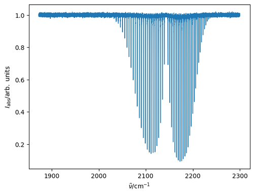
After some imports, we will plot the fundamental infrared absorption band of \(\mathrm{^{12}C^{16}O}\).

import numpy as np
from scipy.signal import find_peaks
import matplotlib.pyplot as plt

# Load the 0-1 spectrum as a function of wavenumber.
nu_v01, Iabs_v01 = np.loadtxt('CO-v01.txt', unpack=True)

plt.plot(nu_v01, Iabs_v01, lw=1)
plt.xlabel(r'$\tilde{\nu}/\mathrm{cm^{-1}}$')
plt.ylabel('$I_\mathrm{abs}/\mathrm{arb.\;units}$')

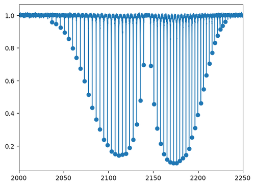
We can use scipy.signal.find_peaks to identify the transition wavenumbers as the centres of each peak in the spectrum. Since the spectrum is measured in absorption, the peaks present as local minima, so we need to find the maxima in the negative of the spectrum array, -Iabs_v01. There is some noise, but with a little trial-and-error we can find suitable parameters prominence and width to pass to scipy.signal.find_peaks in order to capture most of the signals:

idx, _ = find_peaks(-Iabs_v01, prominence=0.04, width=5)
nu_peaks_v01, I_peaks_v01 = nu_v01[idx], Iabs_v01[idx]

plt.plot(nu_v01, Iabs_v01, lw=1)
plt.xlim(2000, 2250)
plt.scatter(nu_peaks_v01, I_peaks_v01)

These absorption lines are usually labelled by the lower-state rotational quantum number: \(P(J'')\) and \(R(J'')\). We could assign the peaks by hand, but the presence of a gap between the \(P(1)\) and \(R(0)\) lines (where the Q-branch, corresponding to \(\Delta J = 0\) transitions is missing for this type of molecule) suggests an automated approach: find the maximum spacing between the peaks: the lines to lower wavenumber are \(P(1), P(2), P(3) \ldots\); those at higher wavenumbers are \(R(0), R(1), R(2) \ldots\)

def assign_J(nu_peaks):
    """
    Return arrays Jpp and Jp: rotational quantum numbers for the lower and upper
    states respectively for the vibrational transitions located at the
    wavenumbers nu_peaks.

    """

    npeaks = len(nu_peaks)
    print(npeaks, 'peaks provided to assign')

    # The spacing between consecutive elements in nu_peaks:
    dnu = np.diff(nu_peaks)
    # Find the index of the maximum spacing, corresponding to the band centre.
    idx = dnu.argmax()

    # We will store the rotational quantum numbers in these arrays.
    Jpp = np.empty(npeaks, dtype=int)
    Jp = np.empty(npeaks, dtype=int)

    # P-branch lines: everything up to (and including) idx,
    # decreasing with increasing index (and hence wavenumber).
    Jpp[:idx+1] = np.arange(idx+1, 0, -1, dtype=int)
    Jp[:idx+1] = Jpp[:idx+1] - 1      # P-branch: J' = J"-1
    # R-branch lines: everything from idx to the end of the array,
    # increasing with increasing index (and hence wavenumber).
    n = npeaks - idx - 1
    Jpp[idx+1:] = np.arange(0, n, 1)
    Jp[idx+1:] = Jpp[idx+1:] + 1      # R-branch: J' = J"+1

    return Jpp, Jp

Jpp_v01, Jp_v01 = assign_J(nu_peaks_v01)
print('Jpp:', Jpp_v01)
print('Jp :', Jp_v01)

51 peaks provided to assign
Jpp: [25 24 23 22 21 20 19 18 17 16 15 14 13 12 11 10  9  8  7  6  5  4  3  2
  1  0  1  2  3  4  5  6  7  8  9 10 11 12 13 14 15 16 17 18 19 20 21 22
 23 24 25]
Jp : [24 23 22 21 20 19 18 17 16 15 14 13 12 11 10  9  8  7  6  5  4  3  2  1
  0  1  2  3  4  5  6  7  8  9 10 11 12 13 14 15 16 17 18 19 20 21 22 23
 24 25 26]

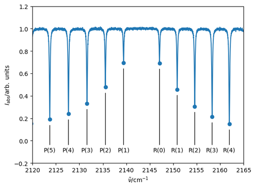
To check we're on the right track, let's produce a labelled spectrum of the region close to the band centre.

plt.plot(nu_v01, Iabs_v01)
xmin, xmax = 2120, 2165
plt.xlim(xmin, xmax)
plt.scatter(nu_peaks_v01, I_peaks_v01)
idx = np.where((xmin < nu_peaks_v01) & (nu_peaks_v01 < xmax))[0]
for i in idx:
    branch = 'P' if Jpp_v01[i] > Jp_v01[i] else 'R'
    # Label the peak with P(J") or R(J") with a line between the label
    # and the peak minimum. shrinkB backs off the line by 10 pts so it doesn't
    # actually connect with the peak: this looks better.
    plt.annotate(f'{branch}({Jpp_v01[i]})', xytext=(nu_peaks_v01[i], -0.1),
                 xy=(nu_peaks_v01[i], I_peaks_v01[i]), ha='center',
                 arrowprops={'arrowstyle': '-', 'shrinkB': 10})
plt.ylim(-0.2,1.2)
plt.xlabel(r'$\tilde{\nu}/\mathrm{cm^{-1}}$')
plt.ylabel('$I_\mathrm{abs}/\mathrm{arb.\;units}$')

We can follow the same process for the first overtone band, using the data in the file CO-v02.txt:

nu_v02, Iabs_v02 = np.loadtxt('CO-v02.txt', unpack=True)
idx, _ = find_peaks(-Iabs_v02, prominence=0.003, width=5)
nu_peaks_v02, I_peaks_v02 = nu_v02[idx], Iabs_v02[idx]

Jpp_v02, Jp_v02 = assign_J(nu_peaks_v02)
print('Jpp:', Jpp_v02)
print('Jp :', Jp_v02)

40 peaks provided to assign
Jpp: [19 18 17 16 15 14 13 12 11 10  9  8  7  6  5  4  3  2  1  0  1  2  3  4
  5  6  7  8  9 10 11 12 13 14 15 16 17 18 19 20]
Jp : [18 17 16 15 14 13 12 11 10  9  8  7  6  5  4  3  2  1  0  1  2  3  4  5
  6  7  8  9 10 11 12 13 14 15 16 17 18 19 20 21]

Fitting the Spectrum

First we need to combine the arrays of peak positions and quantum number assignments:

# All the transitions in a single array.
nu_peaks = np.hstack((nu_peaks_v01, nu_peaks_v02))
# All the lower and upper state rotational quantum numbers.
Jpp = np.hstack((Jpp_v01, Jpp_v02))
Jp = np.hstack((Jp_v01, Jp_v02))
# All the lower and upper state vibrational quantum numbers.
# The bands are 0-1 and 0-2 so the lower state is always v=0.
vpp = np.hstack((np.zeros(Jpp_v01.shape), np.zeros(Jpp_v02.shape)))
# The upper state is v=1 or v=2 for the two bands.
vp = np.hstack((np.ones(Jpp_v01.shape), 2 * np.ones(Jpp_v02.shape)))

Using these arrays, we can build the design matrix, \(\mathbf{X}\), based on the above expression for the transition wavenumbers:

def make_X(vpp, Jpp, vp, Jp):
    return np.vstack(((vp+0.5) - (vpp+0.5),
               (vpp+0.5)**2 - (vp+0.5)**2,
               Jp*(Jp+1) - Jpp*(Jpp+1),
               (vpp+0.5)*Jpp*(Jpp+1) - (vp+0.5)*Jp*(Jp+1),
               (Jpp*(Jpp+1))**2 - (Jp*(Jp+1))**2)).T

X = make_X(vpp, Jpp, vp, Jp)

The fit itself proceeds smoothly:

res = np.linalg.lstsq(X, nu_peaks, rcond=None)
prm_vals = res[0]
sq_resid = res[1]
rank = res[2]
sing_vals = res[3]
print(f'Squared residuals: {sq_resid} cm-1, rms error: {np.sqrt(sq_resid)} cm-1\n'
      f'Rank of X: {rank} (should be = {X.shape[1]})\n'
      f'Singular values of X:{sing_vals}')

Squared residuals: [0.00457467] cm-1, rms error: [0.06763629] cm-1
Rank of X: 5 (should be = 5)
Singular values of X:[2.10195973e+05 3.23559535e+03 1.16404896e+02 3.04587234e+01
 1.95244413e+00]

Note the relatively small residuals: the rms (root-mean-squared) error is a reasonable measure of the goodness of fit. The matrix rank of \(\mathbf{X}\) is the same as the number of parameters to fit, meaning that the model does not contain linearly-dependent terms.

prm_names = ('we', 'wexe', 'Be', 'alphae', 'De')
print(f'The fit parameters (cm-1):')
for prm_name, prm_val in zip(prm_names, prm_vals):
    print(f'{prm_name} = {prm_val:.6g}')

The fit parameters (cm-1):
we = 2169.75
wexe = 13.2396
Be = 1.93137
alphae = 0.0175024
De = 6.20704e-06

These compare quite well to the literature values, based on a more complete fit to a more extensive model function:

\begin{align*} \omega_\mathrm{e} &= 2169.81358\;\mathrm{cm^{-1}}\\ \omega_\mathrm{e}x_\mathrm{e} &= 13.28831\;\mathrm{cm^{-1}}\\ B_\mathrm{e} &= 1.93128087\;\mathrm{cm^{-1}}\\ \alpha_\mathrm{e} &= 0.01750441\;\mathrm{cm^{-1}}\\ D_\mathrm{e} &= 6.12147 \times 10^{-6}\;\mathrm{cm^{-1}} \end{align*}

The fitted parameters can be used to predict the locations of lines that are not observed in the measured spectrum. For example,

def predict(vpp, Jpp, vp, Jp):
    X = make_X(vpp, Jpp, vp, Jp)
    nu_pred = X @ prm_vals
    return nu_pred

# Predict the position of the (0,0) -> (3, 1) line (R(1) of the second overtone):
print(f'nu(0,0 -> 3,1) = {predict(0, 0, 3, 1)} cm-1')

nu(0,0 -> 3,1) = [6354.10656502] cm-1

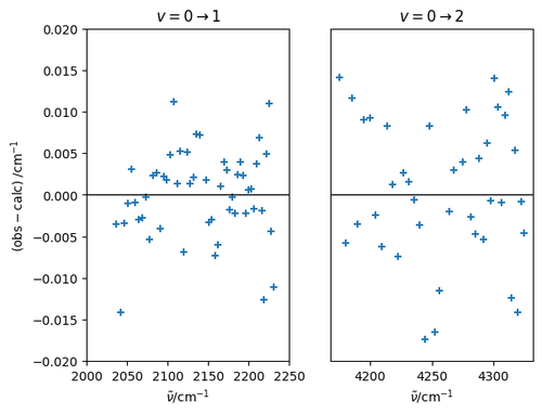
Using this function, the residuals for all of the fitted lines can be plot on a scatter plot.

resid = nu_peaks - predict(vpp, Jpp, vp, Jp)

fig, (ax_v01, ax_v02) = plt.subplots(nrows=1, ncols=2)
ax_v01.scatter(nu_peaks[vp==1], resid[vp==1], marker='+')
ax_v01.set_xlim(2000, 2250)
ax_v01.set_ylim(-0.02, 0.02)
ax_v01.set_xlabel(r'$\tilde{\nu}/\mathrm{cm^{-1}}$')
ax_v01.set_ylabel(r'$\mathrm{(obs - calc)\;/cm^{-1}}$')
ax_v01.axhline(0, c='k', lw=1)
ax_v01.set_title(r'$v = 0 \rightarrow 1$')
ax_v02.scatter(nu_peaks[vp==2], resid[vp==2], marker='+')
ax_v02.set_ylim(-0.02, 0.02)
ax_v02.set_xlabel(r'$\tilde{\nu}/\mathrm{cm^{-1}}$')
ax_v02.set_yticks([])
ax_v02.axhline(0, c='k', lw=1)
ax_v02.set_title(r'$v = 0 \rightarrow 2$')