Which is the most intense line in a rotational spectrum?

Abstract

Most textbooks and lecture notes on molecular spectroscopy assert that the most intense transition in the pure rotational (microwave) absorption spectrum ($J \rightarrow J+1$) of a closed-shell, diatomic molecule is given, as a function of temperature, by the formula

$$ J_\mathrm{max, th} = \sqrt{\frac{T}{2Bc_2}} - \frac{1}{2}, $$

(where $B$ is the molecule's rotational constant and $c_2 = hc/k_\mathrm{B}$). This expression may be readily derived as the most populated rotational level of a rigid rotor. As pointed out by R. J. Le Roy (J. Molec. Spectrosc. 192, 237 (1998)), it is incorrect because it neglects the $J$-dependent Hönl-London factor and stimulated emission ($J+1 \rightarrow J$). A very much better approximation is:

$$ J_\mathrm{max} \approx \sqrt{\frac{3T}{2Bc_2}} - \frac{1}{2} \approx \sqrt{3}J_\mathrm{max,th}, $$

as derived below. Large Language Models (LLMs), such as those employed by ChatGPT, have picked up the incorrect formula, presumably because of the very large corpus of teaching materials available on the internet which use it. This highlights an inherent bias in such LLM tools, which tend to favour the large volume of simplified derivations they encounter in their training set over the more complex, but more rarely-encountered, scientfically accurate derivations.

Derivation

The pure rotational (microwave) absorption spectrum of a closed-shell linear molecule consists of a sequence of lines due to the transitions $J\rightarrow J+1$ which are spaced by roughly $2B$, where $B$ is the rotational constant of the molecule. Various factors lead to these lines varying in intensity but in introductory textbooks and online resources the dominant factor is asserted to be the population of the originating rotational level. The relative population of the rotational level with quantum level is

$$ { f(J) = \frac{2J+1}{q}\exp\left(-\frac{c_2 F(J)}{T}\right), }\tag{1} $$

where $c_2 = hc/k_\mathrm{B} = 1.439\;\mathrm{cm\,K}$ is the second radiation constant and $F(J)$ is the energy of the rotational level with quantum number $J$ in wavenumbers ($\mathrm{cm^{-1}}$); within the rigid rotor approximation,

$$ F(J) = BJ(J+1). $$

The partition function,

$$ q = \sum_{J=0}^\infty (2J+1) \exp\left(-\frac{c_2 F(J)}{T}\right). $$

It is a popular exercise in undergraduate spectroscopy courses to show that the maximum in $f(J)$ is:

$$ J_\mathrm{max, th} = \sqrt{\frac{T}{2Bc_2}} - \frac{1}{2} $$

where $J_\mathrm{max, th}$ is the most populated $J$ level at thermal equilibrium at temperature $T$.

The pure rotational spectrum of CO ($B=1.93\;\mathrm{cm^{-1}}$) at 100 K is shown below.

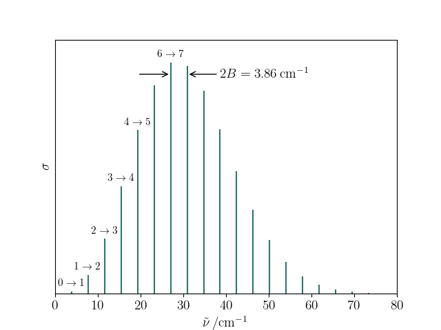
The formula above predicts $J_\mathrm{max, th} = 3.74$ but the most intense line observered is $J = 6 \rightarrow 7$.

def predict_Jmaxth(B, T):
    """Naive prediction of Jmax based on rotational level populations only."""
    return np.sqrt(T / 2 / c2 / B) - 1/2
Jmaxth_100K = predict_Jmaxth(1.93, 100)

The reason for the discrepency is that the transition intensity also depends on other $J$-dependent factors that cannot be ignored when $c_2 B \ll k_\mathrm{B}T$ as is the case for most diatomics at low- to moderate temperatures, including room-temperature. A complete treatment gives

$$ I \propto \frac{J+1}{2J+1} \tilde{\nu}(J) f(J) \left[ 1 - \exp\left( -\frac{c_2\tilde{\nu}(J)}{T}\right)\right], \tag{2} $$

which includes a Hönl-London rotational line strength factor, a dependence on the transition wavenumber, $\tilde{\nu}(J)$, and on the population difference between the upper and lower levels of the transition. This is important because both levels will be appreciably populated and a photon that can induce absorption from $J\rightarrow J+1$ can also induce stimulated emission from $J+1\rightarrow J$. What is observed in the absorption spectrum is the net difference between these processes.

A much more accurate expression was provided by R. J. Le Roy¹ in a 1998 paper which makes for frustrating reading because of some omitted steps and unstated assumptions. The derivation below hopefully fills in some of these gaps.

We start with the rigid rotor approximation expressions for $F(J) = BJ(J+1)$ and

$$ \tilde{\nu}(J) = F(J+1) - F(J) = 2B(J+1). $$

The net absorption intensity can then be written as

$$ I = C (J+1)^2 \exp\left( -\frac{BJ(J+1)c_2}{T}\right) \left[ 1 - \exp\left( -\frac{2B(J+1)c_2}{T}\right)\right], \tag{3} $$

where $C$ is a constant independent of both $J$ and $T$. We are after the maximum in this function of $J$ for a given temperature, so need to find where $\mathrm{d}I/\mathrm{d}J=0$.

Le Roy appears to start by dividing both sides of this equation by $\left[ 1 - \exp\left( -2B(J+1)a\right)\right]$ (where $a=Bc_2/T$ for notational convenience) and carrying out the implicit differentiation:

$$ \begin{align*} & \frac{I}{\left[ 1 - \exp\left( -2(J+1)a\right)\right]} = C(J+1)^2\exp\left( -J(J+1)a\right)\\ \Rightarrow \;\;& \frac{\mathrm{d}I/\mathrm{d}J}{\left[ 1 - \exp\left( -2(J+1)a\right)\right]} - 2aI\left[ 1 - \exp\left( -2(J+1)a\right)\right]^{-2}\exp\left( -2(J+1)a\right) =\\ & \quad\quad -C(J+1)^2a\exp\left( -J(J+1)a\right) + 2C(J+1)\exp\left( -J(J+1)a\right). \end{align*} $$

This is a bit of a mess, but we can make life easier by defining $x=J(J+1)a$ and $y=2(J+1)a$. Setting $\mathrm{d}I/\mathrm{d}J=0$ and using the definition of $I$ then gives:

$$ \begin{align*} &-2aC(J+1)^2e^{-x}\frac{1-e^{-y}}{(1-e^{-y})^{2}}e^{-y} = -C(J+1)^2a(2J+1)e^{-x} + 2C(J+1)e^{-x}\\ \Rightarrow \;\; & \frac{2a(J+1)}{e^y-1} = (J+1)(2J+1)a - 2 \end{align*} $$

This is easier to relate to $J_\mathrm{max,th}$ if we multiply through by $(2J+1)$ and divide by $J+1$:

$$ (2J+1)^2a = \frac{2(2J+1)}{J+1} + \frac{2a(2J+1)}{e^y-1}, $$

which simplifies to

$$ (2J+1)^2a = 4 -\frac{2}{J+1} + \frac{2a(2J+1)}{\exp{[2a(J+1)]}- 1} \tag{4} $$

This is to be solved for $J$ to find $J_\mathrm{max}$. In the low temperature limit, ($a\gg 1$), the last term on the righthand side is negligible and, assuming the second term to be approximately 2, since J approaches 0 in this limit, $(2J+1)^2a \approx 2$ can be rearranged to regain $J_\mathrm{max,th}$.

However, it is more common that $a \ll 1$ since the rotational spacing ($\sim hcB$) is less than $k_\mathrm{B}T$ except for the lightest molecules or at elevated temperatures (for example, in flames). In this case it is helpful to expand the exponential in equation (4) as a Taylor series:

$$ \frac{2(2J+1)a}{\exp{[2a(J+1)]}-1} \approx \frac{2(2J+1)a}{1+2a(J+1) + \frac{4}{2}(J+1)^2a^2-1} = \frac{2J+1}{(J+1)}\frac{1}{[1+(J+1)a]} $$

Further expanding $[1+(J+1)a]^{-1}$ in a Taylor series gives:

$$ \frac{2(J+1)-1}{(J+1)}[1 - (J+1)a] = 2 - (2J+1)a - \frac{1}{J+1} $$

and therefore:

$$ (2J+1)^2a \approx 6 -\frac{3}{J+1} - (2J+1)a \tag{5} $$

With some rearrangement,

$$ \begin{align*} & (2J+1)^2a = \frac{6}{a}\left[1 -\frac{1}{2(J+1)} - \frac{(2J+1)a}{6}\right]\\ \Rightarrow \;\; & J_\mathrm{max} \approx \sqrt{\frac{3}{2a}}\left( 1 - \frac{1}{2(J+1)} - \frac{(J+\frac{1}{2})a}{3}\right)^{1/2} - \frac{1}{2}\\ \Rightarrow \;\; & J_\mathrm{max} \approx \sqrt{\frac{3}{2a}} - \frac{1}{2} \approx \sqrt{3}J_\mathrm{max,th}. \end{align*} $$

The code below compares the actual most intense CO line with that predicted by the formulas $J_\mathrm{max}$ and $J_\mathrm{max,th}$. The experimental data are obtained from the HITRAN files CO-rot.par (line list) and CO-q.txt (partition function).

import marimo as mo
import numpy as np
import pandas as pd
import matplotlib.pyplot as plt
from matplotlib import rc
from scipy.constants import h, c, k as kB
from scipy.interpolate import interp1d
from scipy.optimize import newton
c2 = h * c * 100 / kB   # Second radiation constant, cm.K
rc('font', **{'family': 'serif', 'serif': ['Computer Modern'], 'size': 14})
rc('text', usetex=True)

class ParMeta:
    widths = (2, 1, 12, 10, 10, 5, 5, 10, 4, 8, 15, 15, 15, 15, 6, 12, 1, 7, 7)
    names = ('molec_id', 'iso_id', 'nu', 'S', 'A', 'gamma_air', 'gamma_self',
             'Epp', 'n_air', 'delta_air', 'Vp', 'Vpp', 'Qp', 'Qpp', 'Ierr',
             'Iref', 'flag', 'gp', 'gpp')
    dtypes = {0: int, 1: int, 2: np.float64, 3: np.float64, 4:np.float64,
              5: np.float64, 6: np.float64, 7: np.float64, 8: np.float64,
              9: np.float64, 10: str, 11: str, 12: str, 13: str,
              14: str, 15: str, 16: str, 17: np.float64, 18: np.float64}
    Tref = 296

    def __init__(self):
        pass

    def read_par(self, par_name):
        df = pd.read_fwf(par_name, widths=self.widths, header=None, names=self.names,
                 delim_whitespace=True, dtype=self.dtypes)
        return df

def read_q(q_filename):
    Tgrid, qgrid = np.loadtxt(q_filename, unpack=True)
    q = interp1d(Tgrid, qgrid)
    return q(ParMeta.Tref), q

par_meta = ParMeta()
par_df = par_meta.read_par('CO-rot.par')
qref, q = read_q('CO-q.txt')

def get_Jmaxobs(T):
    S = (
        par_df['S'].values
         * qref / q(T)
         * np.exp(-c2 * par_df.Epp.values / T)
         / np.exp(-c2 * par_df.Epp.values / ParMeta.Tref)
         * (1 - np.exp(-c2 * par_df.nu.values / T))
         / (1 - np.exp(-c2 * par_df.nu.values / ParMeta.Tref))
        )
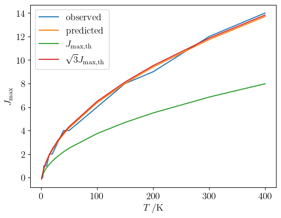
    return np.argmax(S)

A comparison can then be made between the observed $J_\mathrm{max}$ and that predicted by the "thermal" formula, $J_\mathrm{max, th}$ and by the more accurate expression for $J_\mathrm{max}$ derived above.

# Rotational constant for CO
B = 1.93128087
J = np.linspace(0, 51, 52, dtype=int)
F = B * J * (J+1)
J = J[:-1]
Tgrid = np.array([1,2,3,5,8,10,15,20,30,40,50,100,150,200,300,400])
a = c2 * B / Tgrid

def get_Jmaxth(a):
    return np.sqrt(1/2/a) - 1/2

def get_Jmax(a):
    def g(J):
        y = 2 * a * (J+1)
        return 4 - 2 / (J+1) - (2*J+1)**2 * a + 2*a*(2*J+1) * np.exp(-y) / (1-np.exp(-y))
    return newton(g, 10)

Jmaxth = get_Jmaxth(a)
Jmax = np.empty((len(Tgrid)))
Jmaxobs = np.empty((len(Tgrid)))
for i, T in enumerate(Tgrid):
    Jmaxobs[i] = get_Jmaxobs(T)
    Jmax[i] = get_Jmax(a[i])

fig, ax = plt.subplots()
ax.plot(Tgrid, Jmaxobs, label=r"observed")
ax.plot(Tgrid, Jmax, label=r"predicted")
ax.plot(Tgrid, Jmaxth, label=r"$J_\mathrm{max,th}$")
ax.plot(Tgrid, np.sqrt(3) * Jmaxth, label=r"$\sqrt{3}J_\mathrm{max,th}$")
ax.set_xlabel(r'$T\,/\mathrm{K}$')
ax.set_ylabel(r'$J_\mathrm{max}$')
plt.legend()

The predictions made considering the lower level population only are consistently too small by a factor of $\sqrt{3}$.