Fitting the heat capacity curve of a diatomic molecule
The molar constant-pressure heat capacity, \(C_{p,\mathrm{m}}\) of many diatomic molecules above room temperature shows an increase from roughly \(\frac{7}{2}R\) to around \(\frac{9}{2}R\) and then higher as temperature increases. For example the graph below plots \(C_{p,\mathrm{m}}\) as a function of $T$ for the molecules \(\mathrm{N_2}\), \(\mathrm{CO}\), \(\mathrm{HCl}\), \(\mathrm{NO^+}\).
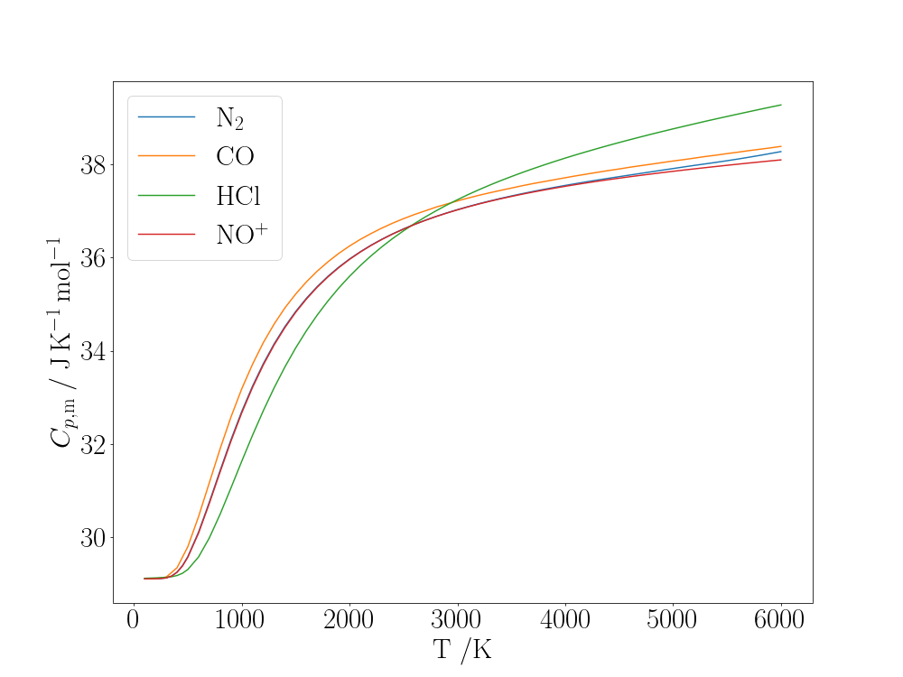
The gaseous constant-pressure heat capacities of some diatomic molecules
At room temperature and above the heat capacity of molecules can be described by classical theory for their translational and rotational motion since their quantum levels are closely-spaced relative to $k_\mathrm{B}T$. As gas molecules, they have three translational degrees of freedom, and as linear molecules they have two rotational degrees of freedom. Rotation around the internuclear axis is neglected since the nuclei are small enough that they can be considered point-masses on the axis and the off-axis electrons are very light. According to equipartition theory, each degree of freedom contributes \(\frac{1}{2}R\) to the heat capacity; there is an additional source of heat capacity in the expansion work that a gas can do at constant pressure, which is accounted for by an extra term \(R\): \(C_{p,\mathrm{m}} = \frac{3}{2}R + \frac{2}{2}R + R = \frac{7}{2}R = 29.1\;\mathrm{J\,mol^{-1}\,K^{-1}}\).
For strongly-bound molecules with high vibrational frequencies, \(h\nu \gg k_\mathrm{B}T\) at room temperature and almost all molecules are in their ground vibrational state ($v=0$) so vibration does not contribute to the heat capacity. As $T$ increases, the excited vibrational states become increasingly accessible and the heat capacity rises. The high-temperature, equipartition limit for the vibrational contribution to the heat capacity is \(R\) (there are two degrees of freedom from the kinetic and potential energy of the single vibrational mode), and so the molar heat capacity is expected to tend towards \(\frac{9}{2}R = 37.4\;\mathrm{J\,mol^{-1}\,K^{-1}}\).
Where deviations from this behaviour occur in some molecules, it is usually because of anharmonicity, unusually widely-spaced rotational levels (\(\mathrm{H_2}\)), low-lying electronic states or a non-closed shell ground state (\(\mathrm{O_2}\), \(\mathrm{NO}\)) or relatively low dissociation energy of the molecule (\(\mathrm{I_2}\)).
For friendly molecules such as \(\mathrm{N_2}\) it should be possible to estimate the vibrational wavenumber, \(\tilde{\nu}\), by fitting the heat capacity as a function of temperature to a model derived from statistical mechanics. Within the harmonic approximation, we start from the vibrational partition function:
$$ q_\mathrm{vib} = \sum_v \exp\left(-\frac{\theta_\mathrm{vib}}{T} v \right) = \frac{1}{1 - \exp\left(-\frac{\theta_\mathrm{vib}}{T}\right)} $$
where $\theta_\mathrm{vib} = hc\tilde{\nu} / k_\mathrm{B}$ and the vibrational energy levels, $\theta_\mathrm{vib} k_\mathrm{B} v = hc\tilde{\nu} v$ for $v=0, 1, \ldots$ are measured relative to the ground state.
The vibrational energy can be obtained from the partition function:
\begin{align*} U_\mathrm{vib, m}(T) &= U_\mathrm{vib, m}(0) + \frac{RT^2}{q_\mathrm{vib}} \frac{\mathrm{d}q_\mathrm{vib}}{\mathrm{d}T}\\ &= U_\mathrm{vib,m}(0) + \frac{\theta_\mathrm{vib} R}{1 - \exp \left( \frac{\theta_\mathrm{vib}}{T} \right)}. \end{align*}
The vibrational contribution to the heat capacity can be derived from the above expression:
$$ C_\mathrm{vib,m} = \frac{\mathrm{d}U_\mathrm{vib,m}}{\mathrm{d}T} = R\left( \frac{\theta_\mathrm{vib}}{T} \right)^2 \frac{\exp \left( \frac{\theta_\mathrm{vib}}{T} \right)}{\left( 1 - \exp \left( \frac{\theta_\mathrm{vib}}{T} \right) \right)^2}. $$
The function to be fit to the above heat capacity curves is therefore
$$ C_\mathrm{tot,m} = \frac{7}{2}R + R\left( \frac{\theta_\mathrm{vib}}{T} \right)^2 \frac{\exp \left( \frac{\theta_\mathrm{vib}}{T} \right)}{\left[ 1 - \exp \left( \frac{\theta_\mathrm{vib}}{T} \right) \right]^2}. $$
Using the heat capacity of \(\mathrm{N_2}\), given in the file N2_Cp.csv, as an example, the scipy.optimize.curve_fit routine can be used to perform this (nonlinear fit):
import numpy as np
from scipy.constants import h, c, k as kB, R
# The second radiation constant, cm.K-1
c2 = h * c * 100 / kB
from scipy.optimize import curve_fit
import matplotlib.pyplot as plt

# Read in the heat capacity as a function of temperature.
T, Cp = np.genfromtxt('N2_Cp.csv', delimiter=',', skip_header=1, unpack=True)

def Cp_SHO(T, theta_vib):
    """Heat capacity including vibration using the SHO model."""
    x = theta_vib / T
    fac = np.exp(x)
    return 7 * R / 2 + R * x**2 * fac / (fac - 1)**2

# Initial guess for the vibrational wavenumber, cm-1.
nu0 = 2000
theta_0 = nu0 * c2
# Fit the Cp data to the harmonic model function.
popt, pcov = curve_fit(Cp_SHO, T, Cp, p0=theta_0)
theta_fit = popt[0]
nu_fit = theta_fit / c2
nu_fit2157.095760135524The fitted vibrational wavenumber is therefore \(2157.1\;\mathrm{cm^{-1}}\).
The data and fit can be plotted with Matplotlib:
plt.plot(T, Cp, '+', label="Experiment")
plt.plot(T, Cp_SHO(T, theta_fit), label="Fit")
plt.xlabel(r"T /K")
plt.ylabel(r"$C_{p,\mathrm{m}} \; / \; \mathrm{J\,K^{-1}\,mol^{-1}}$")
ax.legend()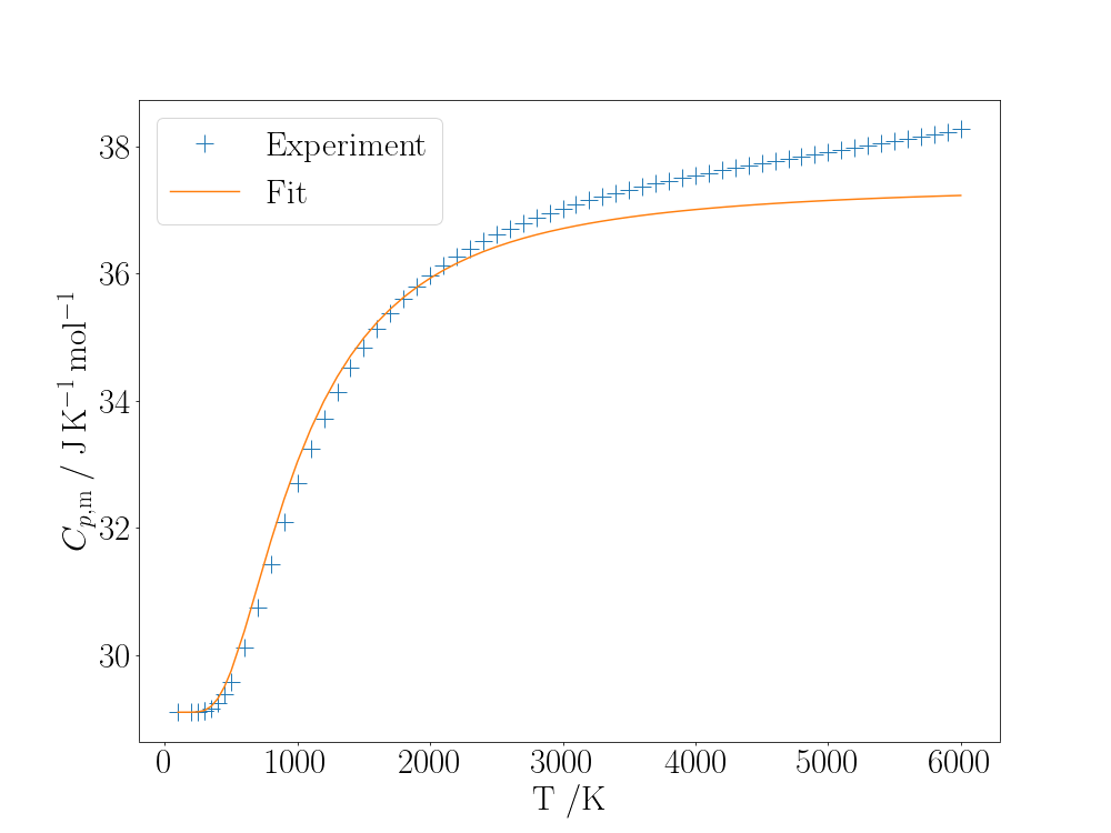
The constant-pressure heat capacity for $\mathrm{N_2}$ and fit to a model treating the vibrational motion as harmonic.
The fit is not particularly good, especially at higher temperatures where several vibrational levels are accessible and anharmonicity leads to closer level spacing than predicted by the harmonic model and hence higher heat capacity.
A better model function to fit would account for anharmonicity in the vibration and for this a more general function is needed. With the following notation:
\begin{align*} q &= \sum_v \exp\left( - \frac{E_v}{k_\mathrm{B}T}\right),\\ \dot{q} &= \frac{\mathrm{d}q}{\mathrm{d}T} = \sum_v \frac{E_v}{k_\mathrm{B}T^2} \exp\left( - \frac{E_v}{k_\mathrm{B}T}\right), \\ \ddot{q} &= \frac{\mathrm{d}^2q}{\mathrm{d}T^2} = \sum_v \frac{E_v}{k_\mathrm{B}T^3} \left( \frac{E_v}{k_\mathrm{B}T} - 2 \right) \exp\left( - \frac{E_v}{k_\mathrm{B}T}\right), \end{align*}
the following expressions can be written:
$$ U_\mathrm{vib,m}(T) = U_\mathrm{m}(0) + RT^2 \left( \frac{\dot{q}}{q} \right) $$
$$ C_\mathrm{vib,m} = \frac{\mathrm{d}U_\mathrm{vib,m}}{\mathrm{d}T} = 2RT\left( \frac{\dot{q}}{q} \right) + RT^2 \left[ \frac{\ddot{q}}{q} - \left(\frac{\dot{q}}{q}\right)^2 \right]. $$
\begin{align*} C_\mathrm{vib,m} &= \frac{\mathrm{d}U_\mathrm{vib,m}}{\mathrm{d}T} = \frac{\mathrm{d}}{\mathrm{d}T} \left[ U_\mathrm{m}(0) + RT^2 \left( \frac{\dot{q}}{q} \right) \right] \\ &= 2RT\left( \frac{\dot{q}}{q} \right) + RT^2 \left[ \frac{q\ddot{q} - \dot{q}\dot{q}}{q^2} \right]\\ &= 2RT\left( \frac{\dot{q}}{q} \right) + RT^2 \left[ \frac{\ddot{q}}{q} - \left(\frac{\dot{q}}{q}\right)^2 \right]. \end{align*}
The code below fits the parameters of the anharmonic vibrational energy described by the power series
$$ \frac{1}{hc}\left(E_v + E_0\right) = \omega_\mathrm{e}\left(v + \frac{1}{2}\right) - \omega_\mathrm{e}x_\mathrm{e}\left(v + \frac{1}{2}\right)^2 + \omega_\mathrm{e}y_\mathrm{e}\left(v + \frac{1}{2}\right)^3 + \omega_\mathrm{e}z_\mathrm{e}\left(v + \frac{1}{2}\right)^4. $$
vmax = 40
def Evib(v, we, wexe=0, weye=0, weze=0):
    """Return the vibrational energy in cm-1."""
    # The zero-point (ground state, v=0) energy.
    E0 = we / 2 - wexe / 4 + weye / 8 + weze / 16
    vph = v + 0.5
    return vph * (we - vph *(wexe - vph * (weye + vph * weze))) - E0

def qvib(T, we, wexe=0, weye=0, weze=0):
    """
    Return the vibrational partition function at temperature T
    and its first and second derivatives.
    """
    q = qdot = qddot = 0
    v = 0
    while v < vmax:
        E = Evib(v, we, wexe, weye, weze)
        x = E * c2
        fac = np.exp(-x / T)
        q += fac
        qdot += x / T**2 * fac
        qddot += x / T**3 * fac * (x / T - 2)
        v += 1
    return q, qdot, qddot

def Cp_anharmonic(T, we, wexe=0, weye=0, weze=0):
    """Return the heat capacity with anharmonic vibration."""
    q, qdot, qddot = qvib(T, we, wexe, weye, weze)
    return 7 * R / 2 + 2 * R * T * qdot/q + R * T**2 * (qddot/q - (qdot/q)**2)

# For this fit, use only the parameters we and wexe (Morse oscillator).
# Initial guess parameters: we, wexe (in cm-1).
p0 = (2000, 10)
popt, pcov = curve_fit(Cp_anharmonic, T, Cp, p0=p0)
popt
array([2354.34692287, 27.41997625])That is, \(\omega_\mathrm{e}=2354.3\;\mathrm{cm^{-1}}\) and \(\omega_\mathrm{e}x_\mathrm{e}=27.4\;\mathrm{cm^{-1}}\), to be compared with the literature values of \(2358.57\;\mathrm{cm^{-1}}\) and \(14.324\). The agreement in the value obtained for \(\omega_\mathrm{e}\) is very good, whilst that for \(\omega_\mathrm{e}x_\mathrm{e}\) is too large by a factor of 2.
The fitted heat capacity curve is this time much better:
plt.plot(T, Cp, '+', label="Experiment")
plt.plot(T, Cp_anharmonic(T, *popt), label="Fit")
plt.xlabel(r"T /K")
plt.ylabel(r"$C_{p,\mathrm{m}} \; / \; \mathrm{J\,K^{-1}\,mol^{-1}}$")
plt.legend()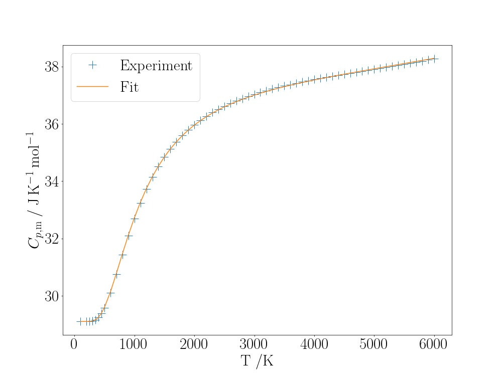
A fit to the temperature-dependence of the constant-pressure heat capacity of $\mathrm{N_2}$ treating its vibration as anharmonic.