A simple plot with pyplot

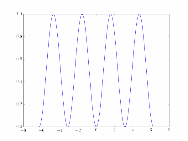
As a simple example of the benefit of using pyplot, let's plot the function $y = \sin^2 x$ for $-2\pi \le x \le 2\pi$. Using only native Python methods, here is one approach:

We calculate and plot 1000 $(x,y)$ points, and store them in the lists ax and ay. To set up the ax list as the abcissa, we can't use range directly because that method only produces integer sequences, so first we work out the spacing between each $x$ value as $$ \Delta x = \frac{x_\mathrm{max} - x_\mathrm{min}}{n-1} $$ (if our $n$ values are to include $x_\mathrm{min}$ and $x_\mathrm{max}$, there are $n-1$ intervals of width $\Delta x$); the abcissa points are then: $$ x_i = x_\mathrm{min} + i\Delta x \quad \mathrm{for}\; i = 0,1,2,\cdots, n-1. $$ The corresponding $y$-axis points are: $$ y_i = \sin^2(x_i). $$ The following program implements this approach, and plots the $(x,y)$ points on a simple line-graph.

import math
import matplotlib.pyplot as plt
xmin, xmax = -2. * math.pi, 2. * math.pi
n = 1000
x = [0.] * n
y = [0.] * n
dx = (xmax - xmin)/(n-1)
for i in range(n):
    xpt = xmin + i * dx
    x[i] = xpt
    y[i] = math.sin(xpt)**2

plt.plot(x,y)
plt.show()

The NumPy equivalents of the math module's methods enable the calculation of y to be vectorized, removing the need for the explicit Python loop. Furthermore, the np.linspace function can be used to create the x array without the need for the above calculation:

import numpy as np
n = 1000
xmin, xmax = -2. * math.pi, 2. * math.pi x = np.linspace(xmin, xmax, n)
y = np.sin(x)**2
plt.plot(x,y)
plt.show()