Learning Scientific Programming with Python (2nd edition)
E8.12: Visualizing the spherical harmonics
Visualising the spherical harmonics is a little tricky because they are complex and defined in terms of angular co-ordinates, $(\theta, \phi)$. One way is to plot the real part only on the unit sphere. Matplotlib provides a toolkit for such 3D plots, mplot3d (see Section 7.6 of the book and the Matplotlib documentation), as illustrated by the code below. Note that the function scipy.special.sph_harm has been replaced by scipy.special.sph_harm_y which takes its arguments in the order: $l$, $m$, $\theta$ and $\phi$.
import matplotlib.pyplot as plt
from matplotlib import cm, colors
from mpl_toolkits.mplot3d import Axes3D
import numpy as np
from scipy.special import sph_harm_y

phi = np.linspace(0, np.pi, 100)
theta = np.linspace(0, 2 * np.pi, 100)
phi, theta = np.meshgrid(phi, theta)

# The Cartesian coordinates of the unit sphere
x = np.sin(phi) * np.cos(theta)
y = np.sin(phi) * np.sin(theta)
z = np.cos(phi)

m, l = 2, 3

# Calculate the spherical harmonic Y(l,m) and normalize to [0,1]
fcolors = sph_harm_y(l, m, theta, phi).real
fmax, fmin = fcolors.max(), fcolors.min()
fcolors = (fcolors - fmin) / (fmax - fmin)

# Set the aspect ratio to 1 so our sphere looks spherical
fig = plt.figure(figsize=plt.figaspect(1.0))
ax = fig.add_subplot(111, projection="3d")
ax.plot_surface(x, y, z, rstride=1, cstride=1, facecolors=cm.seismic(fcolors))
# Turn off the axis planes
ax.set_axis_off()
plt.show()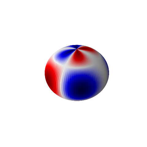
The spherical harmonic Y_32.