Learning Scientific Programming with Python (2nd edition)
P7.7.1: Animating a pendulum
Question P7.7.1
Use Matplotlib's FuncAnimation class to produce an animation of a swinging pendulum with an initial maximum angle from vertical and zero initial velocity. Integrate the equation of motion numerically, and repeat the animation after one period of the motion.
Solution P7.7.1
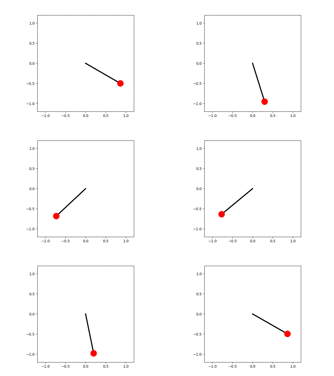
In the code below the equation of motion for the pendulum is solved numerically and each frame of the animation shows an advance of the simulation by a small amount of time, $\mathrm{d}t$. The small-angle approximation for the pendulum's motion gives a lower bound to the period, $$ T_\mathrm{harm} = \frac{1}{2\pi}\sqrt{\frac{L}{g}}. $$ This is used to determine when the pendulum has made one complete swing. The angular positions are calculated for a single period and then used to determine the position of the pendulum bob, which is drawn as a red circle.

A pendulum animation.
import numpy as np
import matplotlib.pyplot as plt
from scipy.special import ellipk
import matplotlib.animation as animation

# Bob mass (kg), pendulum length (m), acceleration due to gravity (m.s-2).
m, L, g = 1, 1, 9.81
# Initial angular displacement (rad), tangential velocity (m.s-1)
theta0, v0 = np.radians(60), 0

# Estimate of the period using the harmonic (small displacement) approximation.
# The real period will be longer than this.
Tharm = 2 * np.pi * np.sqrt(L / g)
# Time step for numerical integration of the equation of motion (s).
dt = 0.001
# Initial angular position and tangential velocity.
theta, v = [theta0], [v0]
old_theta = theta0
i = 0
while True:
    # Forward Euler method for numerical integration of the ODE.
    i += 1
    t = i * dt
    # Update the bob position using its updated angle.
    old_theta, old_v = theta[-1], v[-1]
    omega = old_v / L
    new_theta = old_theta - omega * dt

    # Tangential acceleration.
    acc = g * np.sin(old_theta)
    # Update the tangential velocity.
    new_v = old_v + acc * dt

    if t > Tharm and new_v * old_v < 0:
        # At the second turning point in velocity we're back where we started,
        # i.e. we have completed one period and can finish the simulation.
        break

    theta.append(new_theta)
    v.append(new_v)

# Calculate the estimated pendulum period, T, from our numerical integration,
# and the "exact" value in terms of the complete elliptic integral of the
# first kind.
nsteps = len(theta)
T = nsteps * dt
print(f"Calculated period, T = {T:.4f} s")
print(f"Estimated small-displacement angle period, Tharm = {Tharm:.4f} s")
k = np.sin(theta0 / 2)
Tcalc = 2 * Tharm / np.pi * ellipk(k**2)
print(f"SciPy calculated period, T = {Tcalc:.4f} s")


def get_coords(th):
    """Return the (x, y) coordinates of the bob at angle th."""
    return L * np.sin(th), -L * np.cos(th)


# Initialize the animation plot. Make the aspect ratio equal so it looks right.
fig = plt.figure()
ax = fig.add_subplot(aspect="equal")
# The pendulum rod, in its initial position.
x0, y0 = get_coords(theta0)
(line,) = ax.plot([0, x0], [0, y0], lw=3, c="k")
# The pendulum bob: set zorder so that it is drawn over the pendulum rod.
bob_radius = 0.08
circle = ax.add_patch(
    plt.Circle(get_coords(theta0), bob_radius, fc="r", zorder=3)
)
# Set the plot limits so that the pendulum has room to swing!
ax.set_xlim(-L * 1.2, L * 1.2)
ax.set_ylim(-L * 1.2, L * 1.2)


def animate(i):
    """Update the animation at frame i."""
    x, y = get_coords(theta[i])
    line.set_data([0, x], [0, y])
    circle.set_center((x, y))


nframes = nsteps
interval = dt * 1000
ani = animation.FuncAnimation(
    fig, animate, frames=nframes, repeat=True, interval=interval
)
plt.show()
The output shows the difference between the numerically-integrated, harmonic approximation and calculated values for the pendulum's period:
    Calculated period, T = 2.1550 s
    Estimated small-displacement angle period, Tharm = 2.0061 s
    SciPy calculated period, T = 2.1529 s