Learning Scientific Programming with Python (2nd edition)
E7.7: The one-dimensional diffusion equation
Consider a metal bar of cross-sectional area, $A$, initially at a uniform temperature, $\theta_0$, which is heated instantaneously at the exact centre by the addition of an amount of energy, $H$. The subsequent temperature of the bar (relative to $\theta_0$) as a function of time, $t$, and position, $x$ is governed by the one-dimensional diffusion equation: $$ \theta(x,t) = \frac{H}{c_pA}\frac{1}{\sqrt{Dt}}\frac{1}{\sqrt{4\pi}}\exp\left(-\frac{x^2}{4Dt}\right), $$ where $c_p$ and $D$ are the metal's specific heat capacity per unit volume and thermal diffusivity (which we assume are constant with temperature). The following code plots $\theta(x, t)$ for three specific times and compares the plots between two metals, with different thermal diffusivities but similar heat capacities, copper and iron.
import numpy as np
import matplotlib.pyplot as plt

# Cross sectional area of bar in m3, heat added at x=0 in J
A, H = 1.0e-4, 1.0e3
# Temperature in K at t=0
theta0 = 300

# Metal element symbol, specific heat capacities per unit volume (J.m-3.K-1),
# Thermal diffusivities (m2.s-1) for Cu and Fe
metals = np.array(
    [("Cu", 3.45e7, 1.11e-4), ("Fe", 3.50e7, 2.3e-5)],
    dtype=[("symbol", "|S2"), ("cp", "f8"), ("D", "f8")],
)

# The metal bar extends from -xlim to xlim (m)
xlim, nx = 0.05, 1000
x = np.linspace(-xlim, xlim, nx)

# Calculate the temperature distribution at these three times
times = (1e-2, 0.1, 1)
# Create our subplots: three rows of times, one column for each metal
fig, axes = plt.subplots(nrows=3, ncols=2, figsize=(7, 8))
for j, t in enumerate(times):
    for i, metal in enumerate(metals):
        symbol, cp, D = metal
        ax = axes[j, i]
        # The solution to the diffusion equation
        theta = theta0 + H / cp / A / np.sqrt(D * t * 4 * np.pi) * np.exp(
            -(x**2) / 4 / D / t
        )
        # Plot, converting distances to cm and add some labelling
        ax.plot(x * 100, theta, "k")
        ax.set_title(f"{symbol.decode('utf8')}, $t={t}$ s")
        ax.set_xlim(-4, 4)
        ax.set_xlabel(r"$x\;/\mathrm{cm}$")
        ax.set_ylabel(r"$\Theta\;/\mathrm{K}$")

# Set up the y axis so that each metal has the same scale at the same t
for j in (0, 1, 2):
    ymax = max(axes[j, 0].get_ylim()[1], axes[j, 1].get_ylim()[1])
    print(axes[j, 0].get_ylim(), axes[j, 1].get_ylim())
    for i in (0, 1):
        ax = axes[j, i]
        ax.set_ylim(theta0, ymax)
        # Ensure there are only three y-tick marks
        ax.set_yticks([theta0, (ymax + theta0) / 2, ymax])
# We don't want the subplots to bash into each other: tight_layout() fixes this
fig.tight_layout()
plt.show()
Since Copper is a better conductor, the temperature increase is seen to spread more rapidly for this metal:
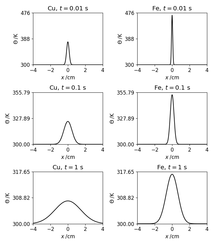
Solution of the one-dimensional diffusion equation for copper and iron.