Learning Scientific Programming with Python (2nd edition)
E7.19: Electrostatic potential of an electric dipole
The following code produces a plot of the electrostatic potential of an electric dipole $\mathbf{p} = (qd, 0, 0)$ in the $(x,y)$ plane for $q=1.602\times 10^{-19}\;\mathrm{C}, d=1\;\mathrm{pm}$ using the point dipole approximation.
import numpy as np
import matplotlib.pyplot as plt

# Dipole charge (C), Permittivity of free space (F.m-1)
q, eps0 = 1.602e-19, 8.854e-12
# Dipole +q, -q distance (m) and a convenient combination of parameters
d = 1.0e-12
k = 1 / 4 / np.pi / eps0 * q * d

# Cartesian axis system with origin at the dipole (m)
X = np.linspace(-5e-11, 5e-11, 1000)
Y = X.copy()
X, Y = np.meshgrid(X, Y)

# Dipole electrostatic potential (V), using point dipole approximation
Phi = k * X / np.hypot(X, Y) ** 3

fig, ax = plt.subplots()
# Draw contours at values of Phi given by levels
levels = np.array([10**pw for pw in np.linspace(0, 5, 20)])
levels = sorted(list(-levels) + list(levels))
# Monochrome plot of potential
ax.contour(X, Y, Phi, levels=levels, colors="k", linewidths=2)
plt.show()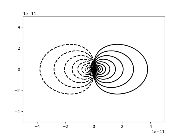
A contour plot of the electrostatic potential of a point dipole.