Visualizing the bivariate Gaussian distribution

$$ p(\boldsymbol{x}; \boldsymbol{\mu}, \boldsymbol{\Sigma}) = \frac{1}{\sqrt{(2\pi)^n|\boldsymbol{\Sigma}|}} \exp\left( -\frac{1}{2}(\boldsymbol{x}-\boldsymbol{\mu})^\mathrm{T}\boldsymbol{\Sigma}^{-1}(\boldsymbol{x}-\boldsymbol{\mu})\right), $$

where $\boldsymbol{\mu}$ is the $n$-dimensional mean vector and $\boldsymbol{\Sigma}$ is the $n \times n$ covariance matrix.

To visualize the magnitude of $p(\boldsymbol{x}; \boldsymbol{\mu}, \boldsymbol{\Sigma})$ as a function of all the $n$ dimensions requires a plot in $n+1$ dimensions, so visualizing this distribution for $n>2$ is tricky. The code below calculates and visualizes the case of $n=2$, the bivariate Gaussian distribution.

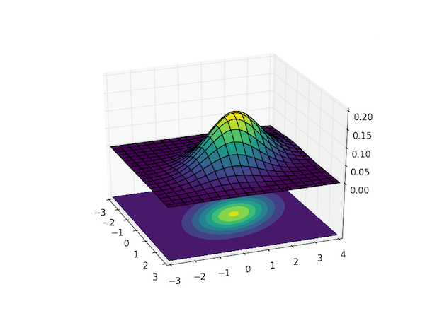
The plot uses the colormap viridis, which was introduced in Matplotlib v.1.4 – you can replace it with any other sane colormap, such as hot if you're on an earlier version of Matplotlib.

import numpy as np
import matplotlib.pyplot as plt
from matplotlib import cm
from mpl_toolkits.mplot3d import Axes3D

# Our 2-dimensional distribution will be over variables X and Y
N = 60
X = np.linspace(-3, 3, N)
Y = np.linspace(-3, 4, N)
X, Y = np.meshgrid(X, Y)

# Mean vector and covariance matrix
mu = np.array([0., 1.])
Sigma = np.array([[ 1. , -0.5], [-0.5,  1.5]])

# Pack X and Y into a single 3-dimensional array
pos = np.empty(X.shape + (2,))
pos[:, :, 0] = X
pos[:, :, 1] = Y

def multivariate_gaussian(pos, mu, Sigma):
    """Return the multivariate Gaussian distribution on array pos.

    pos is an array constructed by packing the meshed arrays of variables
    x_1, x_2, x_3, ..., x_k into its _last_ dimension.

    """

    n = mu.shape[0]
    Sigma_det = np.linalg.det(Sigma)
    Sigma_inv = np.linalg.inv(Sigma)
    N = np.sqrt((2*np.pi)**n * Sigma_det)
    # This einsum call calculates (x-mu)T.Sigma-1.(x-mu) in a vectorized
    # way across all the input variables.
    fac = np.einsum('...k,kl,...l->...', pos-mu, Sigma_inv, pos-mu)

    return np.exp(-fac / 2) / N

# The distribution on the variables X, Y packed into pos.
Z = multivariate_gaussian(pos, mu, Sigma)

# Create a surface plot and projected filled contour plot under it.
fig = plt.figure()
ax = fig.gca(projection='3d')
ax.plot_surface(X, Y, Z, rstride=3, cstride=3, linewidth=1, antialiased=True,
                cmap=cm.viridis)

cset = ax.contourf(X, Y, Z, zdir='z', offset=-0.15, cmap=cm.viridis)

# Adjust the limits, ticks and view angle
ax.set_zlim(-0.15,0.2)
ax.set_zticks(np.linspace(0,0.2,5))
ax.view_init(27, -21)

plt.show()

The matrix multiplication in the exponential is achieved with NumPy's einsum method. The single call:

fac = np.einsum('...k,kl,...l->...', pos-mu, Sigma_inv, pos-mu)

fac = np.einsum('ijk,kl,ijl->ij', x-mu, Sigma_inv, x-mu)

fac = np.einsum('ijk,kl->ijl', pos-mu, Sigma_inv)
fac = np.einsum('ijk,ijk->ij', fac, pos-mu)

The first call here is simply the dot product of the $n_x \times n_y \times 2$ array pos-mu and the $2 \times 2$ covariance matrix Sigma_inv (it could be replaced with np.dot(pos-mu, Sigma_inv)) and results in another $n_x \times n_y \times 2$ array. This is really a $n_x \times n_y$ matrix of vectors, and NumPy has a hard time taking the appropriate dot product with another $n_x \times n_y$ matrix of vectors, pos-mu: we want a matrix of vector dot products, not a vector of matrix dot products. einsum allows us to explicitly state which indexes are to be summed over (the last dimension, indicated by the repeated k in the string of subscripts 'ijk,ijk->ij').

Note: Since SciPy 0.14, there has been a multivariate_normal function in the scipy.stats subpackage which can also be used to obtain the multivariate Gaussian probability distribution function:

Comments

Comments are pre-moderated. Please be patient and your comment will appear soon.

Santhos kumar 4 years, 8 months ago

can we plot two normal surfaces in same graph

Link | Reply

christian 4 years, 8 months ago

Do you mean the sum of two normal surfaces? Sure – just define Z = multivariate_gaussian(pos1, mu1, Sigma1) + multivariate_gaussian(pos2, mu2, Sigma2)

For a stack of surfaces, you'd need to alter the code a bit.

Boimans 4 years, 5 months ago

Great explanation. But I would love to take it a step further. How would I plot a conditional distribution (say one of the x vars = -1) on the same 3D plot? Like this: https://www.researchgate.net/profile/Matthew_Piggott2/publication/318429539/figure/fig1/AS:614381096284160@1523491276935/Linking-two-points-using-a-bivariate-Gaussian-distribution-enables-the-conditional-pdf_W640.jpg

christian 4 years, 4 months ago

If you only want something illustrative, you could get the index of the X coordinate value closest to your desired value (here, 19) and do something like:

ax.plot(np.ones(N)*X[0,19], Y[:,19], Z[:,19], lw=5, c='r', zorder=1000)

You'll need to set the zorder way up because of all those patches.